Spectrogram 🔒
License Required: The Spectrogram window requires a valid LinFIR license.
The Spectrogram visualises the time-frequency energy distribution of the impulse response as a 2-D colour map, making it easy to spot resonances, ringing, and temporal smearing that are difficult to see in a standard frequency response plot.
- Loudspeaker Design mode — shows the predicted sum impulse response for the currently selected angle (on-axis by default); when a non-zero angle is selected in the angle selector the spectrogram updates to reflect that off-axis response, and the window title shows the active angle (e.g. Spectrogram — Predicted Sum — +15°H +0°V)
- Room Calibration mode — shows the averaged measurement impulse response
Accessing the Spectrogram
Menu: View → Spectrogram Keyboard shortcut: W
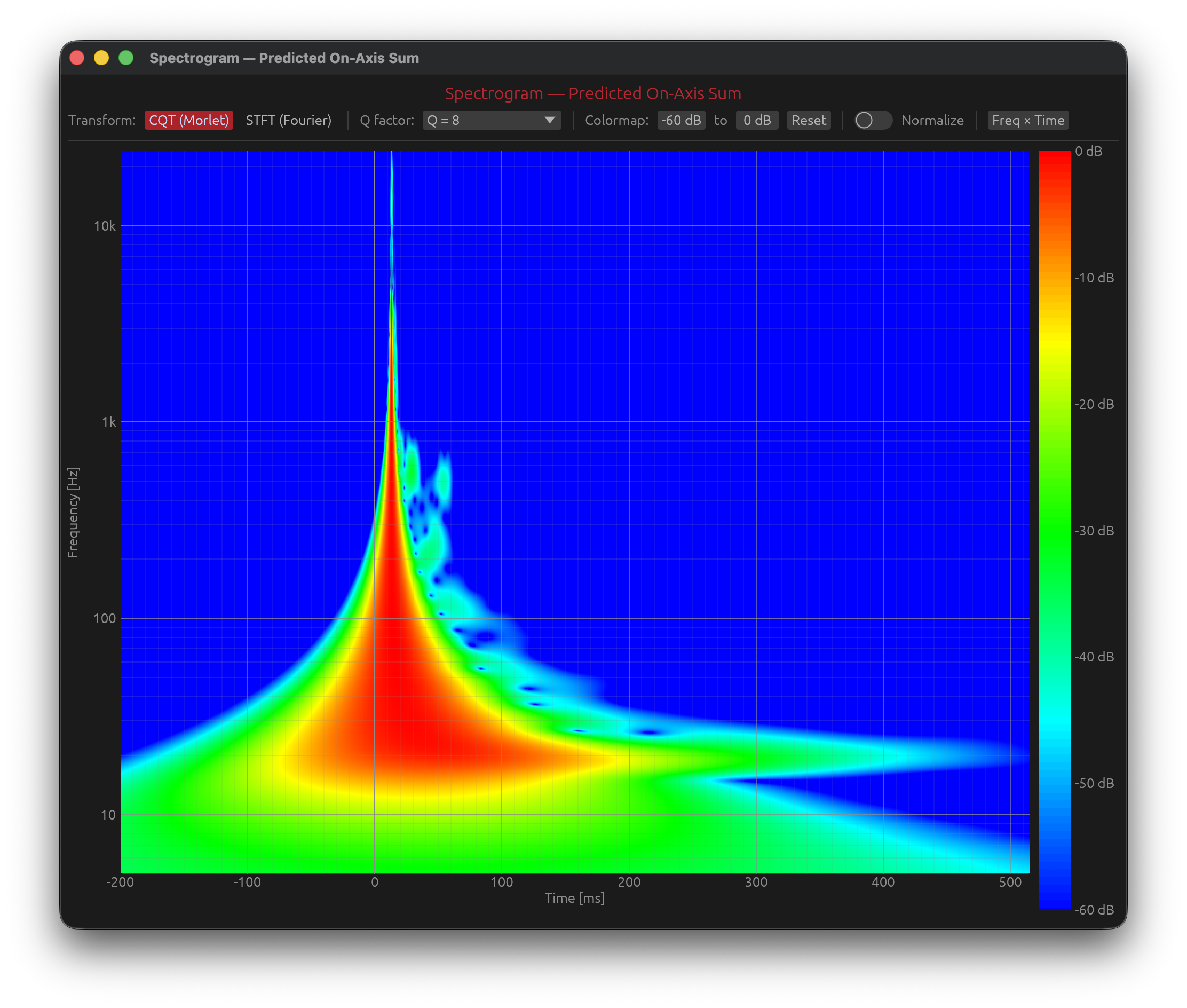
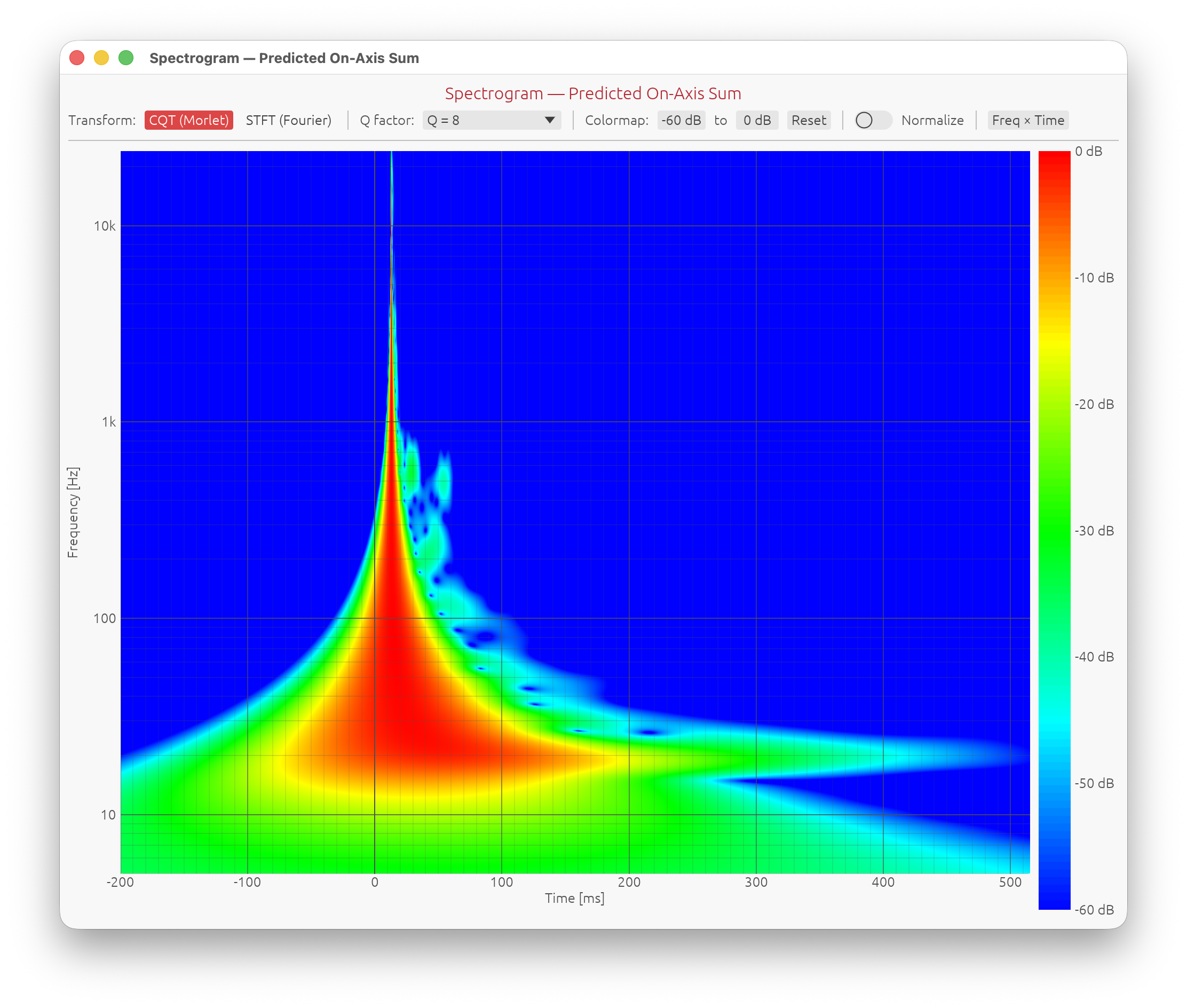
Layout
The window is divided into two panels:
- Main plot — the colour-mapped spectrogram
- Colorbar (right edge) — dB scale matching the current colormap range
A control bar above the plot exposes all parameters.
Controls
Transform Algorithm
Four algorithms are available, selectable from the Transform dropdown:
CQT — Constant-Q Transform (default)
Implemented as a frequency-domain Morlet (analytic Gaussian) filter bank:
- The IR is forward-FFT’d once into an analytic spectrum.
- For each log-spaced frequency f₀, the spectrum is multiplied by a Gaussian window of relative bandwidth 1/Q and inverse-FFT’d.
- The magnitude of the result is the instantaneous amplitude (envelope) at f₀.
This gives constant relative bandwidth — better frequency resolution at low frequencies and better time resolution at high frequencies — which matches the logarithmic frequency axis used throughout LinFIR.
STFT — Short-Time Fourier Transform
A windowed STFT (75% overlap) with linear frequency bins interpolated onto the log display grid. Provides uniform frequency resolution across the spectrum; the Window size controls the time/frequency trade-off and the Shape dropdown chooses the window function (see Window Type).
CSD — Cumulative Spectral Decay
The impulse response progressively truncated from the front: for each of a series of gate positions the IR from that point to the end is transformed, so each slice is the spectrum of the whole remaining tail (only the front of the window moves — a true cumulative decay). The gate’s leading edge is Blackman-Harris tapered. Shows how the spectrum decays over time in milliseconds — the classic tool for spotting loudspeaker resonances. See CSD.
Burst Decay
The same Morlet filter bank as the CQT, but each band’s decay is read on a period-based time axis (t·f). A resonance that rings for N cycles then looks identical at every frequency, so resonances are directly comparable regardless of where they sit — this matches how we hear them (Fryer & Toole). See Burst Decay.
All four modes get a 1 ms raised-cosine fade-out on the end of the impulse response before the transform, so the hard cut where the measurement stops doesn’t smear a broadband click across the last millisecond of the plot.
Resolution Preset
A ComboBox selects the resolution preset for the active algorithm:
| Algorithm | Preset controls | Effect |
|---|---|---|
| CQT | Q factor (4 – 64) | Higher Q → sharper frequency bands, longer time smear |
| STFT | Window size in samples (64 – 32768) | Larger window → better frequency resolution, worse time resolution |
| Burst Decay | Analysis bandwidth (1/3 – 1/24 oct) | Narrower → resolves closer resonances, but the wavelet itself rings longer, raising the analysis floor |
CSD has no resolution preset — its FFT is sized automatically to the length of the impulse-response tail, so low frequencies are never truncated (see CSD).
The Reset button at the end of the first control-bar row returns every mode’s processing parameters (Q factor, Window, Bandwidth, Shape, Rise, Freq res, Pts/period) to their defaults — it leaves the transform mode, the crop/Periods, the frequency range, colormap range, axis layout and toggles alone. The crop/Periods has its own separate Reset, on the row below (see Time crop).
The time–frequency trade-off
Any time-frequency transform faces a fundamental constraint: you cannot simultaneously have perfect time resolution and perfect frequency resolution. Improving one always degrades the other. This is the acoustic equivalent of the Heisenberg uncertainty principle.
CQT Q factor
The Q factor defines the ratio of centre frequency to bandwidth for each analysis band:
$$Q = \frac{f_0}{\Delta f}$$
A band centred at \(f_0=1000, \text{Hz}\) with \(Q = 10\) has a bandwidth of \(\Delta f = 100,\text{Hz}\). The corresponding time resolution (temporal smear) is approximately:
$$\Delta t \approx \frac{Q}{f_0} = \frac{1}{\Delta f}$$
| Q | Frequency resolution | Time resolution | Typical use |
|---|---|---|---|
| 4 – 8 | Coarse | Sharp — short smear | Transient analysis, impact events |
| 12 – 24 | Moderate | Moderate | General loudspeaker IRs (default Q = 12) |
| 32 – 64 | Fine | Blurred — long smear | Resonance identification, room modes |
Because the CQT uses a constant relative bandwidth, low frequencies always have more time smear than high frequencies — this is physically correct and matches how we perceive sound.
STFT window size
The STFT divides the IR into short overlapping frames of fixed length N (in samples). Within each frame, the spectrum is computed with a uniform frequency resolution of \(\Delta f = f_s / N\):
$$\Delta t = \frac{N}{f_s}, \quad \Delta f = \frac{f_s}{N}$$
| Window | Δf at 48 kHz | Δt | Typical use |
|---|---|---|---|
| 128 – 512 | 375 – 94 Hz | 1 – 11 ms | Fast transients, HF detail |
| 1024 – 2048 | 47 – 23 Hz | 21 – 43 ms | Balanced (default) |
| 4096 – 8192 | 12 – 6 Hz | 85 – 170 ms | Fine frequency detail, room modes (default 8192) |
Unlike the CQT, the STFT resolution is the same at all frequencies — which can make low-frequency detail easier to read at the cost of poor high-frequency time resolution.
Detail
Settings → Graphs → Spectrogram detail sets the size of the compute grid — the number of frequency bins and time points the transform is calculated on before it is sampled onto the image:
| Setting | Grid | Notes |
|---|---|---|
| Standard | 2048² | Lightest — the pre-1.4.x behaviour |
| High (default) | 4096² | ~2–4× the compute time, visibly sharper |
| Ultra | 8192² | ~4× the compute time and ~256 MB per recompute — fast machines only |
Higher detail matters most together with the time crop (below), which keeps that grid focused on the part of the response that actually carries signal.
Window Type
For STFT, the Shape dropdown chooses the window function applied to each frame before its FFT. It trades time localisation against spectral leakage (how much a single tone’s energy spreads into neighbouring bins):
| Shape | Character |
|---|---|
| Rectangular | No taper — sharpest time localisation, worst leakage (tall sidelobes) |
| Hann | Good general-purpose low-leakage window |
| Hamming | Like Hann with a raised floor — better nearest-sidelobe rejection |
| Blackman-Harris | Very low sidelobes, at the cost of a wider main lobe |
| Tukey | Flat middle, cosine-tapered ends — between Rectangular and Hann |
| Gaussian | Very low sidelobes (default) |
CQT has no Shape control — its Gaussian is a frequency-domain bandpass shape defining Q, not a time-domain analysis window.
Colormap Range
| Control | Description |
|---|---|
| Min dB (drag-value) | Lower saturation — anything at or below this level renders as cold blue |
| Max dB (drag-value) | Upper saturation — anything at or above this level renders as hot red |
| Reset button | Restores min to the configured default (−30 dB) and max to 0 dB |
Narrowing the range highlights low-level detail (resonances, room modes, late decay). Widening it shows the full dynamic range at a glance.
The Min dB value the window opens with (and that Reset restores) is set by Settings → Graphs → Spectrogram → Spectrogram lower bound, −30 dB by default. It also drives the automatic time crop.
Frequency Range
| Control | Description |
|---|---|
| Frequency (drag-values) | The Min / Max Hz the transform runs on |
| Reset button | Restores both to the current Settings → Graphs values |
This sits on its own control-bar row together with the time crop / Periods controls, below the transform / preset / processing-parameters row — its own Reset button is separate from that row’s processing-parameters one.
Changing either value forces a full recompute — unlike the colormap range, the frequency range is baked into the transform grid, not just the colour mapping. The recompute starts when you release the drag-value, not on every step of the drag.
When a spectrogram cannot be computed - for example an STFT window longer than the impulse response, a minimum frequency too close to the Nyquist limit, or an invalid (all-zero or NaN) response - the window says why instead of showing Computing indefinitely.
This control is independent of Settings → Graphs → Frequency Axis (10 Hz – 24 kHz by default) once set: it is seeded from there when the spectrogram window is first opened, but afterwards changing the Settings value does not silently override it — only its own Reset button pulls the Settings value back in. Every other frequency-axis graph (Magnitude, Phase, Group Delay, HD, the Directivity Sonogram) has no such override and always tracks the Settings value directly.
Normalize
The Normalize toggle scales each frequency band independently so its peak amplitude equals 0 dB. It applies to all four transforms and is a free re-render (no recompute).
- Off — the colormap is referenced to the single loudest point in the whole plot. True relative levels; bands with inherently low energy (deep bass, extreme treble) can appear entirely blue.
- On — every band fills the colormap from its own peak (0 dB) down to Min dB, so decay structure is visible across the whole spectrum regardless of each band’s SPL.
The Min dB / Max dB colormap controls still bound the dynamic range shown within the chosen reference.
Smooth
The Smooth dropdown averages the spectrogram across frequency in fractions of an octave — None (default), 1/48, 1/24, 1/12, 1/6, 1/3 octave, or ERB — the same choices as the main graph’s smoothing, but set here independently. It evens out spectral ripple and measurement noise so decay structure and resonances read more clearly; it applies to all four transforms and to both the 2D image and the 3D waterfall, and is a free re-render (no transform recompute). The window is symmetric in log-frequency, so features stay at their true frequency as the smoothing widens. The grey group-delay line is not affected.
Time crop
The time axis is cropped to the part that carries signal: the leading and trailing time columns in which every frequency sits at or below the Min dB level are dropped. It is measured on the rendered spectrogram itself — the exact grid you see — so the edges of the plot land right where the colour reaches the floor.
| Control | What it does |
|---|---|
| Crop | Start / end of the crop, in ms (CQT / STFT / CSD) — the Periods control doubles as this for Burst Decay, see below. |
| Reset | Goes back to auto-detected. Its own button, right next to Crop / Periods — separate from the processing-parameters Reset on the row above, and from Frequency’s own Reset on the same row. |
- Auto (default): recalculated on every recompute, so it follows Min dB and Normalize — lower the floor (or normalise per band) and more of the lead-in and decay tail is kept; raise the floor to crop tighter. Free (no transform recompute) for CQT / STFT / CSD.
- Manual: drag either Crop field (or Periods, for Burst Decay) and it stops auto-adjusting — the exact value you set is what shows, however Min dB or Normalize change, until you hit Reset. Same on/off-then-pinned idiom as a graph’s auto-bounds.
- A 2-column breathing margin is left on each side of the auto-detected range so the content doesn’t touch the very edge.
- The CQT’s low-frequency filter bank has a long impulse response (∝ Q/f), so its energy genuinely stays above the floor for a long time around the arrival — a CQT plot therefore crops far less tightly than an STFT one. For the tightest auto view of a decay, use STFT or raise Min dB (or just crop manually).
Group Delay overlay toggle
The Group delay toggle shows or hides the grey comparison line (see Group Delay Overlay) and its hover readout. It is only available for the CQT and STFT — the transforms that produce a genuine time-frequency map.
CSD
Cumulative Spectral Decay. For each of a sweep of gate positions the impulse response from the gate to its end is FFT’d, and the results are stacked to show the spectrum decaying over time. Gate 0 is the auto-detected acoustic arrival and the whole tail is shown. Only the gate (the front edge) moves — the far edge stays anchored at the end of the IR — so every slice is the spectrum of the whole remaining tail. The FFT is sized automatically to that tail, so low frequencies are never truncated.
| Control | What it does |
|---|---|
| Rise | The taper on the gate’s leading edge, 0.02–500 ms (default 1). It rises to full value at the gate (ramping up over the samples just before it) and trades time resolution for a smoother spectrum per slice. Short = sharp time resolution but more spectral splatter from the hard cut. |
The time axis is in milliseconds from gate 0 (re-zeroed to the arrival), cropped to where the spectrum clears Min dB. There is no group-delay overlay. Because the axis is in milliseconds, a low-frequency resonance with the same Q as a high-frequency one decays over far more of it and looks slower — which is exactly what Burst Decay fixes by switching to a period axis.
Burst Decay
Burst Decay on a period-based time scale. The same Morlet wavelet analysis as the CQT, but the decay of each frequency is read in cycles of that frequency rather than in milliseconds. On this axis a resonance’s decay slope reads its Q directly, identically at every frequency. Period 0 is locked to the peak of the first arrival.
| Control | What it does |
|---|---|
| Bandwidth | The wavelet’s −3 dB relative bandwidth: 1/3, 1/6 (default), 1/12 or 1/24 octave (Morlet q ≈ 7 / 14 / 29 / 58). Narrower resolves closer resonances but the wavelet itself rings for ≈ q/2π·4 periods, which sets the noise floor of the period axis. |
| Freq res | Frequency-grid density, in points per octave (12–96, default 48; 24–96 is the useful range). Fewer points → faster. |
| Periods | Extent of the period axis — this is the time crop for Burst Decay (default: auto). |
| Pts/period | Samples of the decay envelope per period — the smoothness of the period axis (1–96, default 24). Nearly free (just extra reads of the same wavelet output). |
The time axis is in periods; there is no group-delay overlay. The wavelet’s own ramp-up means each band’s energy peaks a few periods in — the decay is what follows. Caveats: below ~40 Hz the analysis is slow and can show artifacts unless the IR is long (≥ 128k samples); resonances with Q < 2 are hard to see; a reflection at delay \(t_d\) shows up as a decay pattern that slides toward higher frequencies (it sits at \(f \cdot t_d\) periods).
Periods is the crop. Unlike CQT / STFT / CSD, where the crop is a free image-level trim on top of a fixed compute range, here the crop is the compute range — periods are genuinely computed one at a time, so cropping earlier means computing less. While auto (the default), the transform runs out to a generous ceiling (120 periods) internally and Periods shows wherever the decay actually clears Min dB — so you’re not computing 120 periods just to look at 20 of them. Drag Periods to pin an exact extent (now a real compute-range change: expect a brief recompute); it stays there — through Min dB, Normalize, anything — until Reset.
Axis Swap
The Freq × Time / Time × Freq button swaps the horizontal and vertical axes:
- Time × Freq (default) — time on X (ms), frequency on Y (Hz, log)
- Freq × Time — frequency on X (Hz, log), time on Y (ms)
Swapping the axes resets the zoom to fit the new layout.
The layout the spectrogram opens with is set by Settings → Graphs → Spectrogram axes; the toolbar button then swaps it for the current session.
3D waterfall
The 2D / 3D button (start of the third control-bar row) switches the main area between the flat colour image and a rotatable 3D surface — the classic waterfall. It works for all four transform modes; the surface is the same time–frequency grid, with height and colour driven by level, using the same colormap and the same Min dB / Max dB, Normalize, and time crop settings as the 2D view — switching between 2D and 3D never changes what range of the decay is shown.
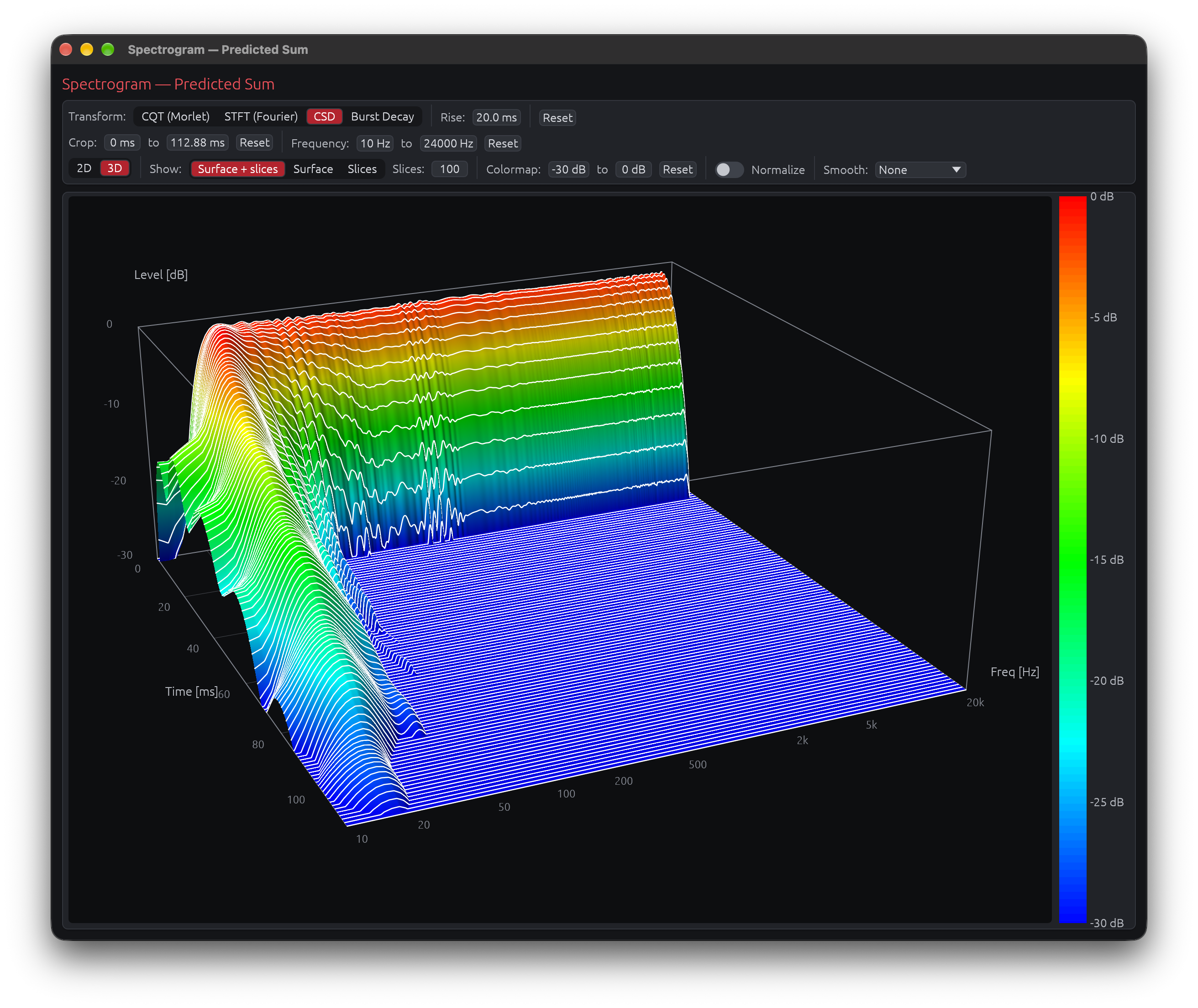
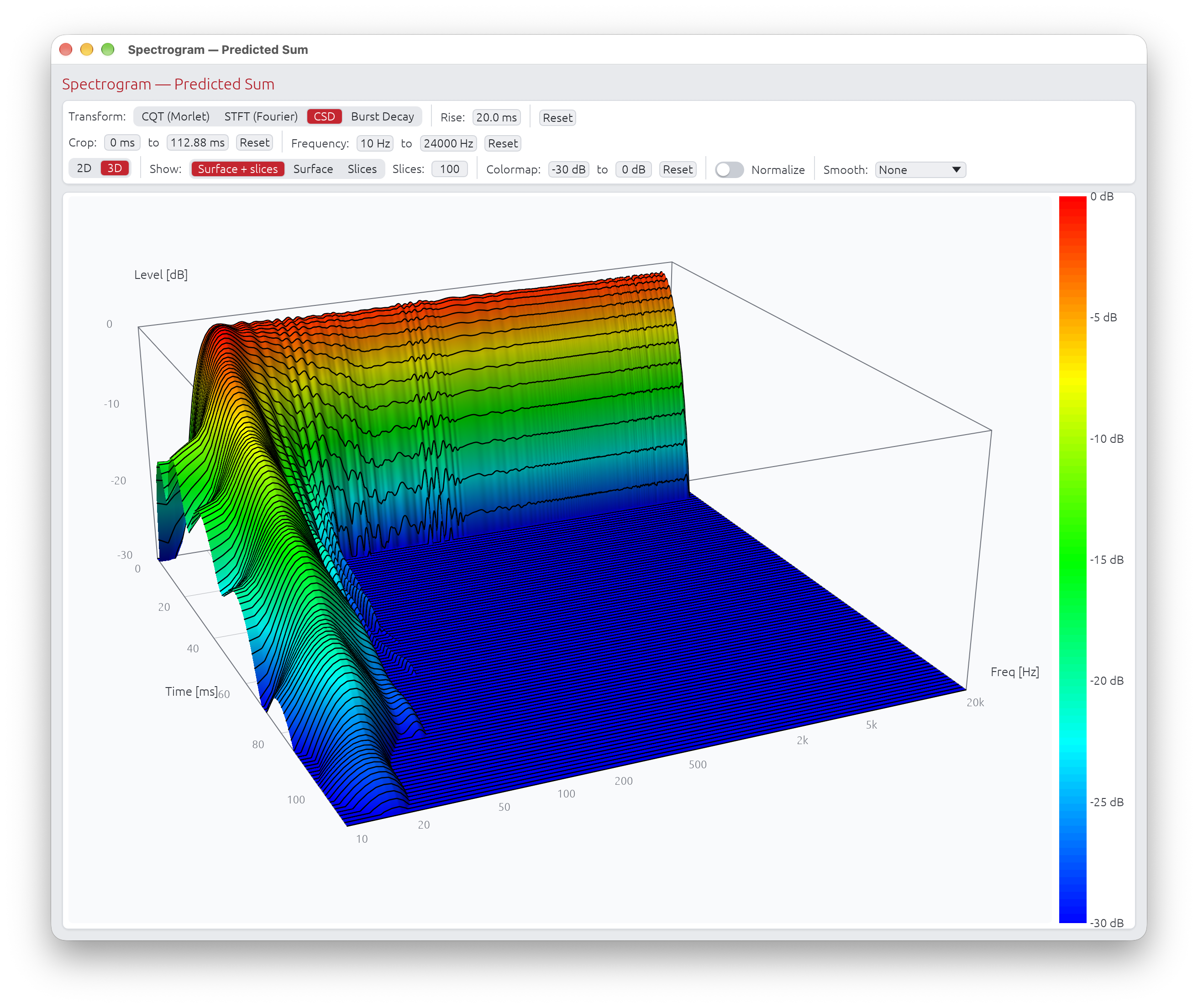
- Left-drag to rotate, right-drag to pan, scroll / pinch to zoom, double-click to reset the view.
- Hover the surface for a readout: the time-slice (spectrum at that instant) and frequency-slice (decay at that frequency) are drawn on the surface where they cross, with a time / frequency / level box at the cursor.
- Show picks what to draw: Surface + slices (default), Surface only, or Slices only — the slices are constant-time (or constant-cycle for burst decay) lines on the surface; Slices sets how many (default 100).
- Switching 2D ↔ 3D is instant — nothing is recomputed.
- In 3D the axis-swap and Group-delay controls are hidden (they don’t apply).
The surface is directionally shaded (a fixed light, upper-left) so ridges and valleys read clearly — colour still encodes level, so a shadowed slope looks darker than the colorbar for the same dB; the hover box gives the exact value. The leading and trailing silence is trimmed the same way as the 2D image (following Min dB).
Group Delay Overlay
A thin grey line traces the group delay across frequency on top of the colour map (toggle it with Group delay in the control bar). It uses the same Smoothing amount as the main window’s Group Delay graph and is shifted by the same Delay Compensation, computed directly from the same impulse response the spectrogram itself displays, so it lines up with the image’s time axis. (The smoothing here is applied per-octave symmetrically, so a bump in the grey line stays at its true frequency instead of drifting down as the smoothing widens.)
This lets you compare the two directly: a resonance or smear visible in the colour map that lines up with a bump in the grey line (e.g. cone breakup, a port or panel resonance) is a genuine group-delay anomaly at that frequency, not just an artifact of the time-frequency transform’s own resolution trade-off.
Hover Tooltip
Hovering the plot shows the time, frequency, and level in dB at the cursor, letting you read a precise value instead of estimating it from the colour.
The tooltip also reports the Group Delay value when the cursor is actually hooking the grey overlay line.
Plot Interaction
| Action | Effect |
|---|---|
| Drag | Pan |
| Scroll / pinch | Zoom |
| Box zoom (right-click drag) | Zoom to selection |
| Double-click | Reset to auto-fit |
After a double-click the view stays in auto-fit: it re-frames itself whenever the image changes (Min dB, transform, axis layout) until you next pan or zoom.
Related Documentation
- Graph Interaction — zoom, pan, and detached windows
- Directivity Analysis — directivity sonogram and overlay plot
- License — license features and activation