Target Curves

Target curves define the desired frequency response for FIR correction and Auto EQ optimization. LinFIR provides built-in curves (Flat, Harman) and supports fully customizable user-defined curves.

Target curves are used by:

• FIR Correction filters (per-driver and global)
• Auto EQ (per-driver and global IIR optimization)

Each filter type has its own independent target curve configuration.

Accessing Target Curve Configuration

Target curve windows are accessed from configuration buttons in the corresponding filter windows:

Per-Driver:

• FIR Correction: Driver → FIR Correction → Magnitude Correction section → Configure button
• Auto EQ: Driver → IIR Filters → Auto EQ tab → Target Curve section → Configure button

Global:

• Global FIR Correction: Global FIR → Magnitude Correction section → Configure button
• Global Auto EQ: Global IIR → Auto EQ tab → Target Curve section → Configure button

Built-in Target Curves

Flat Curve

Description: 0 dB gain across all frequencies (20 Hz to 20 kHz)

Use Cases:

• Anechoic measurements requiring no psychoacoustic compensation
• Verification/troubleshooting (no tonal bias)
• Starting point for custom curves

Initialization:

• Click Flat button
• Creates 2 control points: (20 Hz, 0 dB) and (20 kHz, 0 dB)

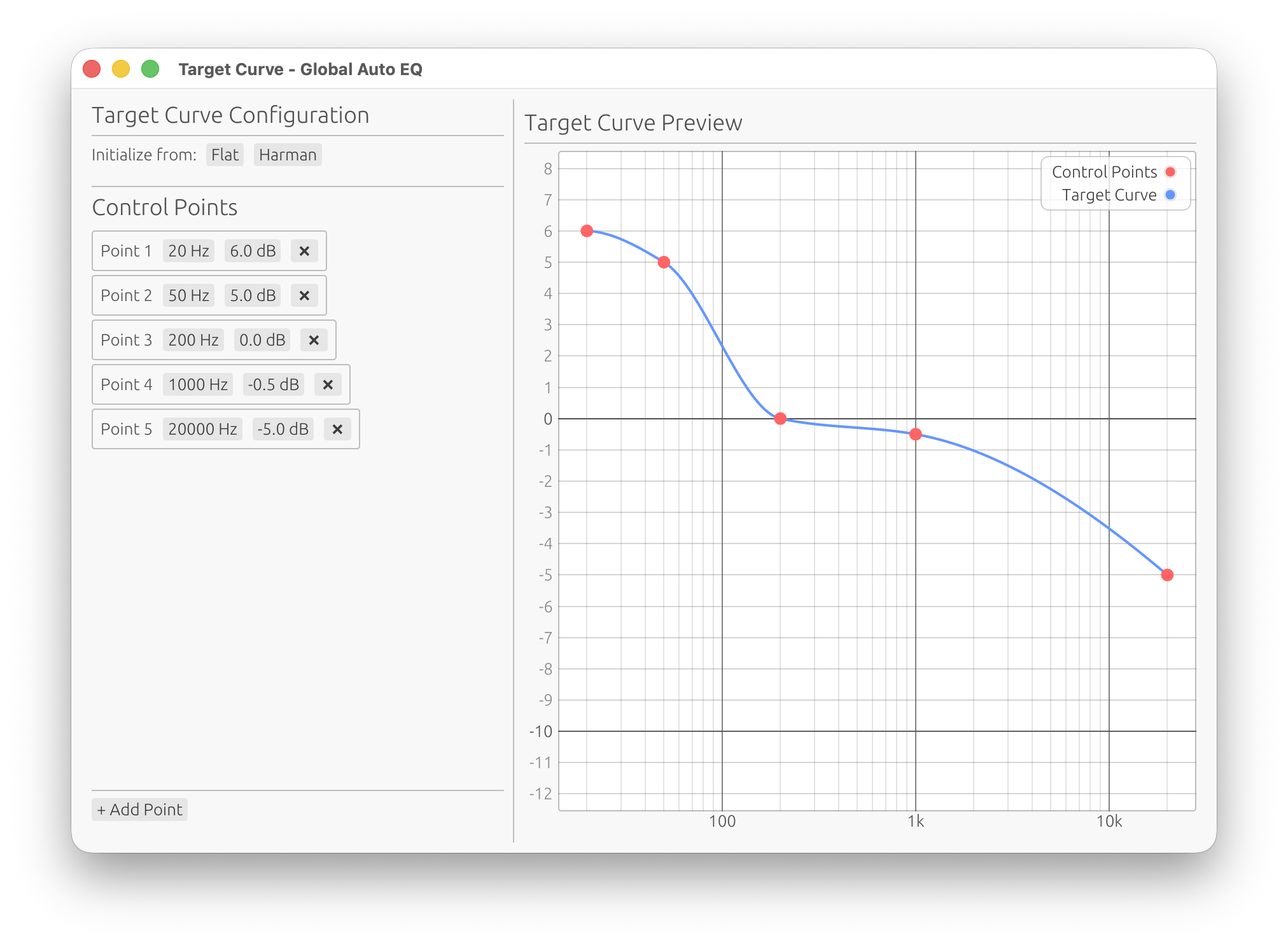
Harman Target Curve

Description: Psychoacoustically optimized frequency response based on Harman research

Curve Shape:

• +6 dB at 20 Hz: Enhanced deep bass presence
• +5 dB at 50 Hz: Bass warmth
• 0 dB at 200 Hz: Neutral lower midrange
• -0.5 dB at 1 kHz: Slight midrange dip (reference frequency)
• -5 dB at 20 kHz: Treble roll-off (reduces harshness)

Use Cases:

• In-room listening: Compensates for typical room gain and psychoacoustic preferences
• Room calibration: Starting point for subjective tuning

Initialization:

• Click Harman button
• Creates 5 control points with Harman curve shape

Customization:

• Adjust bass tilt by modifying low-frequency points
• Adjust treble slope by changing high-frequency points
• Add intermediate points for detailed shaping

⚠️ Critical: Max. Attenuation vs. Curve Amplitude

FIR correction filters work primarily by attenuation (cutting peaks). The Max Attenuation parameter must be large enough to accommodate the amplitude of the target curve within the configured frequency range.

Example (full Harman curve, 20 Hz - 20 kHz): The default Harman curve has an amplitude of 11 dB (from +6 dB at 20 Hz to -5 dB at 20 kHz). If you set Max Attenuation to only 6 dB, the FIR filter cannot apply the full curve—specifically, the treble roll-off (-5 dB at 20 kHz) will not be applied.

Example (limited range, 200 Hz - 20 kHz): If you set Frequency Range from 200 Hz to 20 kHz, the effective amplitude is only 5 dB (from 0 dB at 200 Hz to -5 dB at 20 kHz). In this case, Max Attenuation ≥ 5 dB is sufficient.

Rule: Set Max Attenuation ≥ curve amplitude within f_min to f_max.

• Calculate amplitude: Find max and min gain within your configured frequency range
• Harman (20 Hz - 20 kHz): Use Max Attenuation ≥ 11 dB (recommend 12-15 dB)
• Harman (200 Hz - 20 kHz): Use Max Attenuation ≥ 5 dB (recommend 6-8 dB)
• Custom curves: Calculate max - min within your f_min/f_max range

Applies to: FIR Correction filters (per-driver and global). Auto EQ uses IIR filters (can boost and cut freely).

Custom Target Curves

Create fully custom target curves with unlimited control points.

Control Points

Each control point defines a (frequency, gain) pair:

Frequency:

• Range: 1 Hz to 21,000 Hz
• Log-scale distribution recommended (e.g., 20, 50, 100, 200, 500, 1k, 2k, 5k, 10k, 20k Hz)
• Drag value to adjust

Gain:

• Range: -20 dB to +20 dB
• Positive values = boost, negative = cut
• Drag value to adjust

Minimum Points: 2 (required for interpolation)

Adding Points

1. Click + Add Point button
2. New point created at 1 kHz, 0 dB
3. Adjust frequency and gain as needed

Removing Points

1. Click ❌ button next to the control point
2. Cannot remove if only 2 points remain (minimum requirement)

Curve Interpolation

LinFIR automatically interpolates between control points to create a smooth curve:

Interpolation Process:

1. Generate 5,000 log-spaced frequencies across the full range
2. Log interpolation between user control points onto these 5,000 frequencies
3. Linear interpolation from 5,000 points to target frequencies (filter FFT bins)

Result: Smooth, natural curve without artifacts even with few control points

Preview: Real-time graph shows interpolated curve (blue line) and control points (red dots)

Target Curve Preview Graph

The right panel shows a real-time preview of the target curve.

Elements:

• Blue line: Final interpolated target curve (used by correction algorithms)
• Red dots: User-defined control points

Axes:

• X-axis: Frequency (Hz, logarithmic scale)
• Y-axis: Gain (dB, linear scale)

Auto-scaling: Y-axis automatically adjusts to fit data range

Workflow Recommendations

Creating a Custom Curve from Scratch

1. Click Flat to start with a neutral baseline
2. Add control points at key frequencies:
   • 20 Hz: Deep bass level
   • 50-100 Hz: Bass warmth
   • 200-500 Hz: Lower midrange body
   • 1 kHz: Reference point (usually 0 dB or slightly negative)
   • 2-5 kHz: Presence region
   • 10 kHz: Air/sparkle
   • 20 kHz: Extreme treble roll-off
3. Adjust gains to shape desired response
4. Preview in graph and test with measurements

Modifying Harman Curve

1. Click Harman to load default curve
2. Adjust existing points:
   • Reduce 20-50 Hz gains for less bass
   • Increase 20 kHz gain for more treble extension
   • Add points at 2-5 kHz for presence adjustment
3. Use as starting point for room-specific tuning

Room Calibration Workflow

1. Measure in-room response without any FIR or IIR EQ
2. Start with Harman curve (accounts for typical room gain)
3. Apply correction and re-measure
4. Fine-tune target curve:
   • Reduce bass points if room has excessive low-frequency gain
   • Adjust treble roll-off based on room absorption
   • Add notches at problematic room modes (if using Auto EQ)
5. Iterate until subjectively satisfying

Loudspeaker Design Workflow

1. Use Flat curve for anechoic FIR correction (individual drivers)
2. Measure on-axis response and apply correction
3. Verify off-axis response maintains reasonable shape

Best Practices

Control Point Placement

• Use logarithmic spacing: Match human auditory perception (e.g., 20, 50, 100, 200, 500 Hz…)
• Avoid excessive points: 5-10 points typically sufficient for smooth curves
• Anchor bass and treble: Always define endpoints (20 Hz, 20 kHz)
• Reference at 1 kHz: Many conventions use 1 kHz as 0 dB reference

Curve Shape Considerations

• Avoid steep transitions: Can cause ringing in FIR filters and excessive Q in Auto EQ
• Match measurement reliability: Don’t define detailed curve below measurement noise floor
• Account for driver capabilities: Don’t demand excessive bass from small drivers
• Psychoacoustic balance: Consider Fletcher-Munson curves at typical listening levels

FIR Correction: Max Attenuation vs. Curve Amplitude

Critical requirement for FIR correction filters:

FIR correction works primarily by attenuation (cutting peaks in the frequency response). The Max Attenuation parameter limits how much the filter can cut.

Problem: If the target curve has a large amplitude (difference between highest and lowest points), and Max Attenuation is set too low, the filter cannot apply the full curve shape.

Solution: Set Max Attenuation ≥ curve amplitude within the configured frequency range

Calculating Curve Amplitude:

1. Find the highest gain in your target curve within f_min to f_max (configured Frequency Range)
2. Find the lowest gain in your target curve within f_min to f_max
3. Amplitude = highest - lowest within that range

Examples:

Harman curve, full range (20 Hz - 20 kHz):

• Highest: +6 dB at 20 Hz
• Lowest: -5 dB at 20 kHz
• Amplitude: 6 - (-5) = 11 dB
• Required: Max Attenuation ≥ 11 dB (recommend 12-15 dB)

Harman curve, limited range (200 Hz - 20 kHz):

• Highest: 0 dB at 200 Hz
• Lowest: -5 dB at 20 kHz
• Amplitude: 0 - (-5) = 5 dB
• Required: Max Attenuation ≥ 5 dB (recommend 6-8 dB)

Flat curve (any range):

• Amplitude: 0 dB (curve is flat)
• Any Max Attenuation works

Custom +10 dB bass, -8 dB treble, full range:

• Amplitude: 10 - (-8) = 18 dB
• Required: Max Attenuation ≥ 18 dB (recommend 20 dB)

What happens if Max Attenuation is too low:

• The filter clips the attenuation at the maximum value
• Parts of the curve are not applied (typically treble roll-off is lost)
• Result: Incomplete correction, unbalanced tonal response

Recommendation:

• Calculate amplitude only within your configured f_min/f_max range
• Add 1-3 dB margin above calculated amplitude
• Monitor corrected frequency response to verify full curve is applied
• If limiting frequency range (e.g., 200 Hz - 10 kHz), you may need much less Max Attenuation

💡 Tip: This only applies to FIR correction filters. Auto EQ uses IIR filters which can boost and cut freely, so this limitation does not apply.

Testing and Validation

1. Preview before applying: Check interpolated curve makes sense
2. Apply to measurement: Use with FIR correction or Auto EQ
3. Measure result: Verify corrected response matches target
4. Iterate: Refine target based on measurements and listening tests

Technical Details

Interpolation Algorithm

Step 1: Log-space interpolation

• Creates 5,000 log-spaced frequencies from minimum to maximum input frequency
• Uses logarithmic interpolation between user control points
• Preserves smooth transitions in log-frequency domain

Step 2: Linear resampling

• Resamples 5,000-point curve to target frequencies (FFT bins)
• Linear interpolation ensures smooth curve on target grid
• No artifacts or discontinuities

Result: High-quality curve suitable for both FIR convolution and IIR optimization

Frequency Range

• Minimum: 1 Hz (typically clamp to 20 Hz in practice)
• Maximum: 21,000 Hz (or Nyquist frequency, whichever is lower)
• Interpolation: Extends user points across full range

Gain Limits

• Range: -20 dB to +20 dB per control point
• No hard limit on curve: Interpolation can produce values outside this range between points
• Practical limit: Avoid extreme gains to prevent filter artifacts

Common Use Cases

Studio Monitoring

Target: Custom curve with gentle tilt (or modified Harman)

• Modern practice uses in-room curves rather than flat anechoic response
• Gentle treble roll-off (-1 to -3 dB at 20 kHz) reduces listening fatigue
• Slight bass lift (+1 to +3 dB below 100 Hz) compensates for room interaction
• Purely flat curves are rarely used in practice—can sound harsh and fatiguing
• Start with Harman and adjust to taste for extended listening sessions

Home Theater

Target: Harman curve (or modified)

• Preferred tonal balance for movies and music
• Accounts for room gain
• Adjust bass/treble tilt to taste

Hi-Fi Listening

Target: Custom curve based on Harman

• Start with Harman, adjust to preference
• Reduce bass if room is overly boomy
• Adjust treble based on speaker and room brightness

Car Audio

Target: Custom curve (elevated bass and treble)

• Compensate for road noise (boost bass and treble)
• Account for small cabin gain
• Highly subjective—tune by ear

Headphone Compensation

Target: Diffuse-field or Harman headphone curve

• Compensate for headphone frequency response
• Simulate speaker-like tonality

Related Documentation

• Driver Processing: FIR correction and Auto EQ using target curves
• System Processing: Global FIR correction and Auto EQ

Summary

Target curves define the desired frequency response for correction algorithms:

• Built-in curves: Flat (0 dB) and Harman (psychoacoustic optimized)
• Custom curves: Unlimited control points with automatic interpolation
• Independent configuration: Each FIR correction and Auto EQ has its own target
• Real-time preview: Interactive graph shows interpolated curve

Workflow:

1. Open target curve window from filter configuration (Configure button)
2. Initialize from Flat or Harman, or create custom
3. Add/edit control points (frequency, gain)
4. Preview interpolated curve in real-time
5. Apply correction and measure results
6. Iterate based on measurements and listening tests

Use target curves to shape your system’s tonal balance, compensate for room effects, and achieve your desired sound signature.