Graph Interaction & Display
This section covers all interactive features, display controls, and analysis tools available when working with LinFIR’s graphs.
Graph Toolbar
The graph toolbar provides comprehensive controls for selecting which data to display and how to visualize it. The toolbar adapts based on the project mode (Loudspeaker Design vs Room Calibration).
Loudspeaker Design Mode:


Room Calibration Mode:


Display Mode Selection
Purpose: Choose which stage of the signal processing chain to visualize.
Available modes:
- FIR - FIR filter responses only (crossovers, magnitude/phase correction)
- IIR - IIR filter responses only (parametric EQ, shelves, crossovers)
- FIR+IIR - Combined FIR and IIR responses
- Drivers (Loudspeaker Design) / Measurements (Room Calibration) - Full signal chain applied to driver or room measurements (theoretical system response)
Keyboard shortcuts:
- Press F to cycle through filter modes (FIR → IIR → FIR+IIR)
- Press D to switch to Drivers/Measurements mode
Mode behavior:
- Loudspeaker Design mode: Shows individual driver filters plus global filters
- Room Calibration mode: Shows only global filters in FIR/IIR/FIR+IIR modes
See Display Modes section below for detailed explanations of each mode.
Graph Visibility Toggles — “Graphs” Dropdown
Purpose: Show or hide specific graph types.
Graph types are grouped in the Graphs dropdown in the toolbar. Opening the dropdown reveals toggles for each graph type:
- Magnitude (M) - Frequency response in dB
- Impulse Response (I) - Impulse response in time domain
- Step Response (T) - Step response in time domain
- Group Delay (G) - Group delay in milliseconds
- Phase (P) - Phase response in degrees
- Harmonic Distortion (K) - (Loudspeaker Design / Hypex mode only)
Letters in parentheses indicate keyboard shortcuts. The dropdown stays open when toggling items, allowing multiple graphs to be shown or hidden without reopening it.
Note: Harmonic Distortion is only available in Loudspeaker Design / Hypex mode with Drivers display mode active, as harmonic distortion analysis is not applicable to in-room measurements.
License Feature: The HD graph displays the total harmonic distortion for all users. Individual harmonic curves (\(h_2\), \(h_3\), \(h_4\), \(h_5\)) are only available with a valid license.
Angle Selector (Loudspeaker Design / Hypex mode only)
Purpose: Select which off-axis measurement angle to display when drivers have directivity data.
- Horizontal angles: Typically ±15°, ±30°, ±45°, ±60°, ±75°, ±90°
- Vertical angles: Same as horizontal
- Toggle H/V: Switch between horizontal and vertical axis selection
Only available when at least one driver has off-axis measurements. The selector is hidden in Room Calibration mode as directivity analysis is specific to anechoic/quasi-anechoic loudspeaker measurements.
See Directivity Analysis for complete details on polar measurements and analysis.
Time Domain Options — “Time Domain” Dropdown
The Time Domain dropdown groups options that affect impulse and step response display.
Normalize
Purpose: Scale impulse and step responses to ±1 range for easier comparison.
When enabled:
- Impulse responses normalized to peak amplitude = 1
- Step responses normalized to maximum value = 1
- Useful for comparing relative timing and shape without amplitude differences
Focus on Summed Response
Purpose: Use the time boundaries of the summed impulse response for all IR and step response plots.
- Loudspeaker Design: All time-domain plots are framed around the summed driver output
- Individual curves remain visible within those boundaries
- Useful for evaluating overall system timing alignment
Phase Options — “Phase Options” Dropdown
The Phase Options dropdown is enabled only when the Phase graph is visible. It contains two options:
Unwrap Phase
Purpose: Display continuous phase response without ±180° wrapping discontinuities.
- Disabled: Phase wraps at ±180° (sawtooth pattern)
- Enabled: Phase continues beyond ±180° showing true accumulated phase shift
- Essential for analyzing linear phase filters and group delay
- Makes phase response easier to interpret across wide frequency ranges
Remove time of flight rotations
What is a time of flight? A pure propagation delay — the time it takes for sound to travel from the driver to the measurement microphone — appears in the phase response as a constant linear slope: the further the impulse response peak is from t = 0, the steeper the slope, and the more the phase accumulates rotations across the frequency range. This linear ramp carries no useful information about the filter or driver behaviour; it just reflects the physical distance between source and mic.
This option removes that linear component, leaving only the non-linear phase rotations introduced by the filters and the acoustics of each driver. The result is a much flatter, easier-to-read phase curve, and — when multiple drivers are shown — it becomes straightforward to compare their phase alignment without the bulk delay dominating the picture.
- Disabled: Phase includes the full linear delay component (steep slope proportional to time of flight)
- Enabled: Linear component subtracted, phase flattens around 0° — non-linear deviations stand out clearly
HD Display Mode (Loudspeaker Design mode only)
Purpose: Select how harmonic distortion values are displayed on the HD plot.
Available display modes:
- Percent (%) - Traditional percentage representation
- dB (relative) - Relative level compared to fundamental
- dB (absolute) - Absolute RMS level of harmonics
Percent (%) Mode:
Displays harmonic distortion as a percentage relative to the fundamental (\(h_1\)). Values above 100% are possible when harmonic components exceed the fundamental level (e.g., below the driver’s resonance frequency).
dB (relative) Mode:
Expresses harmonic distortion relative to the fundamental (\(h_1\)) in decibels. Negative values indicate harmonics are quieter than the fundamental; positive values indicate harmonics exceed the fundamental. For example:
- -40 dB ≈ 1% distortion
- -60 dB ≈ 0.1% distortion
- -80 dB ≈ 0.01% distortion
- 0 dB = 100% distortion (harmonics equal the fundamental)
Useful for evaluating signal-to-distortion ratio.
dB (absolute) Mode:
Shows the absolute level of the harmonics alone, without normalization. This mode is useful for comparing distortion levels across different SPL measurements, as it shows the actual acoustic power in harmonic components regardless of the fundamental level.
Individual Harmonics:
All three modes also display individual harmonic curves (\(h_2\), \(h_3\), \(h_4\), \(h_5\)) with dashed/dotted line styles. The selected mode applies to both the total HD curve and individual harmonics.
License Feature: Individual harmonic curves (\(h_2\)-\(h_5\)) are only available with a valid license.
Smoothing
Purpose: Apply smoothing to magnitude, HD, directivity, group delay and phase plots.
Smoothing options:
- None - No smoothing (raw response)
- 1/48 octave - Very fine smoothing
- 1/24 octave - Fine smoothing
- 1/12 octave - Moderate smoothing
- 1/6 octave - Coarse smoothing
- 1/3 octave - Very coarse smoothing
- ERB - Perceptually-motivated variable smoothing (see below)
Applies to:
- Magnitude (frequency response)
- Group delay
- Phase (preserves driver alignment via trend removal method)
- HD (Harmonic Distortion)
- Directivity Analysis (sonogram)
Does not affect: Time-domain plots (impulse, step response)
ERB Smoothing:
ERB (Equivalent Rectangular Bandwidth) smoothing uses a variable bandwidth that corresponds to the frequency resolution of the human auditory system. The smoothing bandwidth follows the formula: (107.77f + 24.673) Hz, where f is frequency in kHz.
This results in:
- Heavy smoothing at low frequencies (~1 octave at 50Hz, 1/2 octave at 100Hz, 1/3 octave at 200Hz)
- Moderate smoothing at mid frequencies (approximately 1/6 octave above 1kHz)
- Natural perceptual weighting that reflects how the ear integrates frequency information
ERB smoothing is particularly useful for:
- Understanding what a listener actually perceives
- Comparing measurements to subjective listening impressions
- Evaluating whether fine response details are audible
Note: Smoothing is cosmetic and does not affect filter calculations or exports. See Fractional Octave Smoothing section below for detailed behavior.
Mouse & Trackpad Controls
Zoom Controls
Zoom In - Multiple methods:
- Box zoom: Right-click and drag to select a region
- Trackpad pinch: Pinch gesture to zoom in/out
- Mouse wheel: Scroll to move the view within a graph
Zoom Out:
- Double-click anywhere on a graph to reset to auto-calculated bounds
- Double-click re-enables auto-bounds mode (graphs automatically adjust to data range)
Pan
Left-click and drag to move the view within a zoomed graph.
Legend Interaction
Click on color dots in the legend to show/hide individual curves:
- Hidden curves are grayed out in the legend
- Click again to show the curve
- Useful for isolating specific drivers or filters
Detach Graphs
Right-click on any graph to open it in a separate window:
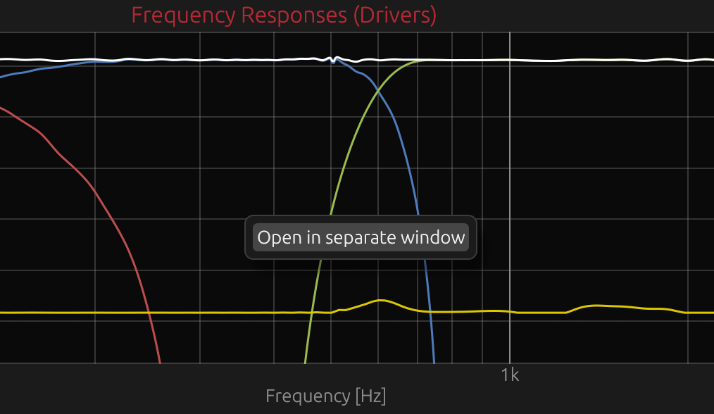
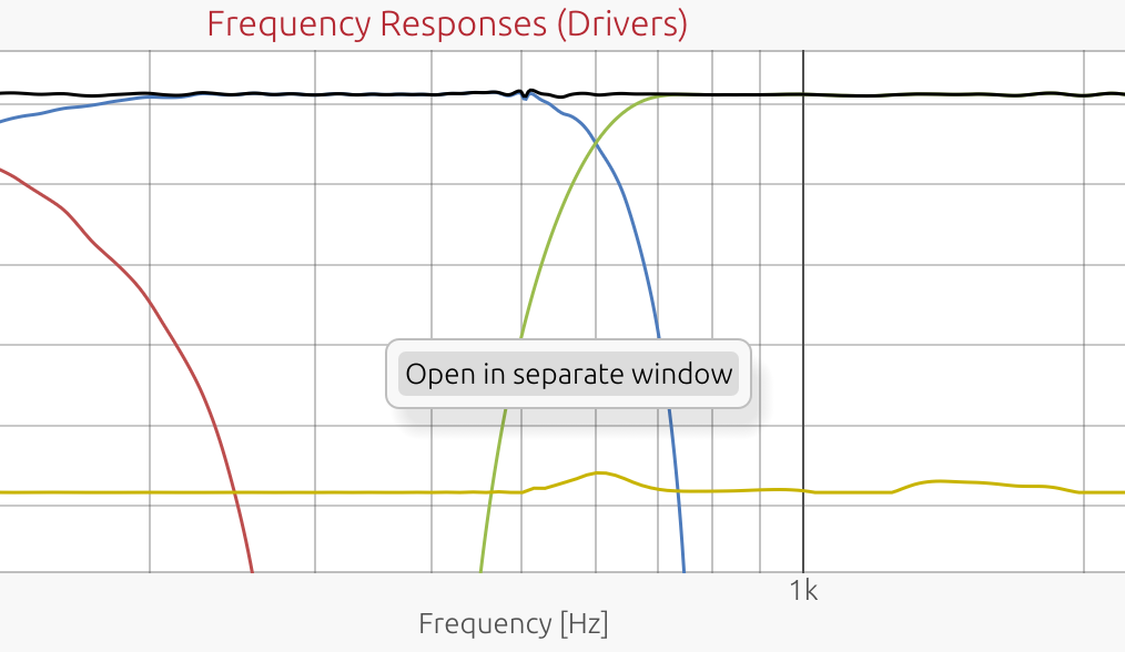
- All graph types supported (Frequency, Phase, Group Delay, Impulse, Step, HD)
- Detached windows render in real-time following the active display mode
- Multiple graphs can be opened simultaneously for side-by-side comparison
- Ideal for multi-monitor setups and detailed analysis workflows
- Close detached windows: Cmd+W (macOS) / Ctrl+W (Windows)
Display Modes
Project Mode Impact
LinFIR supports two project modes that affect display terminology:
- Loudspeaker Design - Speaker design with drivers
- Room Calibration - Multi-position measurements for room correction
In Room Calibration mode:
- “Drivers” mode is renamed to “Measurements”
- Individual measurement curves are shown in Measurements mode
- Filter modes (FIR/IIR/FIR+IIR) display only global filters
In Loudspeaker Design mode:
- “Drivers” mode displays individual drivers
- Filter modes show both per-driver filters and global filters
Filters vs. Drivers/Measurements Mode
Filters Mode (Keyboard: F):
- Shows individual filter responses (FIR, IIR, or FIR+IIR combined)
- Press F multiple times to cycle through filter submodes:
- FIR Filters - Shows only FIR filter responses
- IIR Filters - Shows only IIR filter responses
- FIR+IIR Filters - Shows combined FIR and IIR responses
- Loudspeaker Design: Per-driver crossover and correction filters displayed separately
- Room Calibration: Only global filters are shown
- Global filters shown as additional curves
- Useful for analyzing filter design and frequency response shaping
Drivers/Measurements Mode (Keyboard: D):
- Loudspeaker Design: Shows combined driver + filter responses (acoustic output)
- Each curve represents the complete signal chain for that driver
- Sum curve shows the total system response at listening position
- Room Calibration: Shows individual measurement positions and averaged response
- Each curve represents a raw measurement location (no filters applied)
- Sum curve shows the averaged response with global filters applied
- Useful for analyzing final acoustic performance
Graph Visibility Toggles
Show/hide individual graph types using keyboard shortcuts:
- M - Toggle Magnitude (Frequency Response) plot
- P - Toggle Phase Response plot
- G - Toggle Group Delay plot
- I - Toggle Impulse Response plot
- T - Toggle Step Response plot
- K - Toggle HD (Harmonic Distortion) plot
X-Axis Synchronization
Toggle: X key or toolbar button
When enabled, Sync X-axis synchronizes the horizontal axis across related plots:
Frequency Plots (Magnitude, Phase, Group Delay, Directivity Analysis):
- All plots share the same frequency range
- Zooming any plot updates all frequency plots simultaneously
- Double-click resets all frequency plots to full range
Time Plots (Impulse, Step Response):
- All time-domain plots share the same time range
- Zooming any plot updates all time plots simultaneously
- Double-click resets all time plots to full range
Independent Y-Axes:
- Each plot maintains its own vertical scale
- Y-axis auto-bounds independently for each graph type
Use Cases:
- Compare magnitude and phase behavior at the same frequency
- Analyze impulse and step response in the same time window
- Maintain consistent zoom across multiple graph types
Impulse & Step Response Normalization
Toggle: N key or toolbar button
Normalizes impulse and step responses to peak amplitude = 1.0:
Purpose:
- Allows visual comparison between responses with different amplitudes
- Focuses on filter shape and time-domain characteristics
- Eliminates gain differences for easier visual analysis
Effect:
- All IR and SR curves are scaled to the same peak height
- Does not affect magnitude or phase plots
- Purely visual - does not modify underlying data
Use Cases:
- Compare filter shapes between drivers with different sensitivity
- Analyze time-domain behavior without gain differences obscuring details
- Identify pre-ringing or timing issues across multiple drivers
Focus on Summed Response
Toggle: S key or Time Domain dropdown (Drivers/Measurements mode only)
Synchronizes the time window of all temporal plots (Impulse & Step Response) to the Sum/Average curve boundaries:
How it Works:
- Analyzes the Sum/Average impulse response to find its energy boundaries
- Detects first and last samples above -60 dB threshold (1/1000th of peak)
- Adds configurable margins before and after the detected energy region
- Applies the same time window to all temporal plots (both Impulse and Step Response)
- Enables auto-bounds for all time plots
Behavior:
- Requires at least 2 active curves to activate (otherwise ignored)
- Focuses all temporal plots on the main acoustic energy of the Sum/Average response
- Individual driver/measurement curves are zoomed to the same time window as the sum
- Easier to compare arrival times and transient behavior across all curves
- Works with adaptive display mode margins (configurable in Settings)
Use Cases:
- Loudspeaker Design: Quickly identify timing alignment issues across drivers
- See if all drivers arrive within the sum’s main energy window
- Detect delays or misalignment relative to system response
- Room Calibration: Focus on the averaged room response energy region
- Compare individual measurement positions to the average response timing
- Identify room reflections within the main energy window
- Eliminate clutter from pre-ringing or tail noise outside the main energy region
Only available in Drivers/Measurements Mode (not applicable to individual filters).
Note: Works in both Loudspeaker Design and Room Calibration project modes when display mode is set to Drivers/Measurements.
Phase Display Options
Unwrap Phase
Toggle: U key or toolbar button
Controls phase display format:
Wrapped Phase (default):
- Phase values constrained to ±180°
- Shows discontinuities (phase wraps) at ±180° boundaries
- Easier to read for simple filters
- Standard display format for most audio applications
Unwrapped Phase:
- Continuous phase values extending beyond ±180°
- Shows total accumulated phase shift
- Useful for analyzing group delay trends and overall phase shift
Note: Group delay is always computed from unwrapped phase internally. The Unwrap toggle only affects phase display, not group delay accuracy.
Remove time of flight rotations
Toggle: C key or Phase Options dropdown (next to Unwrap Phase)
A pure propagation delay translates into a linear slope in the phase response — the further the impulse response peak is from t = 0, the steeper the slope, and the more rotations accumulate across the frequency range. This linear ramp is entirely determined by the physical distance between the driver and the microphone and does not reveal anything about filter behaviour or driver characteristics.
This option removes that linear component via a linear regression on the IR peak position, leaving only the non-linear phase introduced by the filters and acoustics. Phase curves become much flatter, easier to read, and directly comparable across drivers regardless of their physical placement.
Removes the linear phase component (constant group delay) from phase responses:
Algorithm:
- Computes linear phase slope from IR peak position for all curves (drivers and filters)
- Subtracts the constant group delay (linear phase shift)
- Flattens phase around 0° while preserving relative phase differences
- Works with both wrapped and unwrapped phase display modes
In Loudspeaker Design Mode (Drivers):
When multiple speakers are active:
- Removes the linear delay of the Sum curve from all responses
- Centers all driver phases around 0° relative to the system response
- Highlights phase alignment issues between drivers
- Makes phase differences visible without bulk delay obscuring them
When single driver is active:
- Removes the linear component of that driver’s phase
- Flattens phase around 0° to show only non-linear phase shifts
In Room Calibration Mode (Measurements):
- Independent correction: Removes the linear phase component of each individual measurement independently
- No shared reference - each measurement position is treated separately
- Flattens each measurement’s phase around 0°
- Useful for comparing phase behavior across different room positions without timing offsets
- The averaged curve also has its own linear component removed
In Filters Mode (FIR, IIR, FIR+IIR):
- Per-filter correction: Removes the linear phase component of each individual filter
- Flattens each filter’s phase around 0°
- Reveals only non-linear phase rotations introduced by the filter
- Useful for analyzing filter phase behavior independent of bulk delay
Use Cases:
- Identify phase alignment issues between drivers without delay obscuring differences
- Visualize phase rotations introduced by filters (independent of linear delay)
- Compare filter phase characteristics across different designs
- Verify minimum-phase vs. linear-phase behavior
Fractional Octave Smoothing
Control: Dropdown menu in toolbar (None, 1/48 oct to 1/3 oct, or ERB)
Apply smoothing to reduce measurement noise and reveal trends:
Fixed Fractional-Octave Smoothing:
- No smoothing - Show raw response (no averaging)
- 1/48 octave - Very fine smoothing (highest detail)
- 1/24 octave - Fine smoothing
- 1/12 octave - Moderate smoothing (default)
- 1/6 octave - Coarse smoothing
- 1/3 octave - Very coarse smoothing (lowest detail)
ERB (Equivalent Rectangular Bandwidth) Smoothing:
ERB smoothing uses a frequency-dependent bandwidth that models the human auditory system’s frequency resolution. Unlike fixed fractional-octave smoothing, ERB adapts its bandwidth at each frequency according to psychoacoustic research.
Bandwidth formula: (107.77f + 24.673) Hz, where f is in kHz
Frequency-dependent behavior:
- 50 Hz → ~1 octave bandwidth (heavy smoothing)
- 100 Hz → ~1/2 octave bandwidth
- 200 Hz → ~1/3 octave bandwidth
- 1 kHz and above → ~1/6 octave bandwidth (leveling out)
When to use ERB smoothing:
- To see what the ear actually perceives (perceptually accurate)
- When evaluating audibility of response features
- To match listening test results with measured data
- For publication-quality graphs that reflect human hearing
When to use fixed fractional-octave smoothing:
- For equalization and correction work (1/6 or 1/12 octave recommended)
- When analyzing crossover behavior in detail
- To maintain consistent resolution across all frequencies
- For technical comparisons between drivers
Effect:
- Wider smoothing = smoother curves, less detail
- Narrower smoothing = more detail, more noise visible
- ERB = perceptually-weighted smoothing (variable with frequency)
Applies to:
- Frequency response (magnitude), HD, Directivity Analysis (sonogram), group delay and phase plots
- Does not affect time-domain plots (impulse responses)
Note: Smoothing is applied after all processing (filters, crossovers, correction). It affects display only, not exported data. It can also alter crossover slopes on the graphs.
Impulse Response Analysis
Automatic Pre-Ringing Detection
When hovering over impulse response curves, LinFIR displays additional analysis information:
Pre-ring Level (in dB relative to peak):
- Weighted RMS measurement of signal energy before the main peak
- Analysis stops at the last zero-crossing before peak (excludes rising edge)
- Uses Hilbert envelope to capture perceptible energy regardless of phase
- Perceptually weighted: energy closer to the peak is less penalized (temporal masking)
- Displayed as:
Pre-ring: -50.0 dB (Likely masked)
Algorithm Details:
- Find the impulse peak position and amplitude
- Find the last zero-crossing before the peak (to exclude the rising edge)
- Extract the pre-ringing region (from start to zero-crossing)
- Calculate the Hilbert envelope of the pre-ringing region
- Apply sigmoid weighting (closer to peak = less perceptual penalty)
- Masking time at 50% penalty: 0.6 ms (default)
- Weight floor: 0.2 (minimum weight for distant pre-ring)
- Weight ceiling: 1.0 (maximum weight for near-peak pre-ring)
- Calculate weighted RMS of the envelope
- Convert to dB relative to peak amplitude
Weighting Rationale:
- Pre-ringing close to the peak is masked by the main transient (temporal masking)
- Pre-ringing far from the peak is more audible (less masking)
- Sigmoid function models gradual transition from masked to unmasked
Risk Assessment Labels
Pre-ringing levels are classified based on typical perceptual thresholds (indicative):
| Level (dB) | Risk Assessment | Description |
|---|---|---|
| ≤ -36 dB | Likely masked | Generally inaudible, masked by main transient |
| -36 to -24 dB | Low risk | May be perceptible in some cases (quiet passages) |
| -24 to -12 dB | Moderate risk | Likely perceptible depending on program material |
| > -12 dB | High risk | Potentially objectionable, consider reducing filter length |
Important Notes:
- These are indicative estimates, not absolute rules
- Actual audibility depends on:
- Program material (transient-rich vs. sustained tones)
- Listening level
- Individual hearing sensitivity
- Room acoustics and background noise
- Use as a guideline for filter design, not strict limits
- Shorter FIR filters or increased causality reduce pre-ringing at the cost of magnitude and phase accuracy
Trade-offs:
- Longer FIR filters → More pre-ringing, better magnitude/phase accuracy
- Shorter FIR filters → Less pre-ringing, reduced correction capability
- Higher causality (e.g., minimum-phase) → Less pre-ringing, potential phase distortion
- Linear-phase (causality = 0) → Maximum pre-ringing, linear phase
Auto-Bounds Behavior
LinFIR automatically adjusts graph bounds to fit data:
Auto-Bounds Enabled (default):
- Graphs automatically scale to show all data
- Y-axis adjusts when switching between drivers or display modes
- X-axis adjusts based on data range (frequency or time)
Auto-Bounds Disabled (after user interaction):
- Manual zoom/pan disables auto-bounds for that axis
- Graph retains user-specified bounds
- Switching modes preserves manual bounds
- Double-click re-enables auto-bounds and resets to calculated range
Per-Axis Independence:
- X-axis and Y-axis auto-bounds are independent
- Dragging vertically disables Y auto-bounds, preserves X auto-bounds
- Dragging horizontally disables X auto-bounds, preserves Y auto-bounds
- Box zoom (right-click drag) disables both X and Y auto-bounds
Per-Graph Independence:
- Each graph type has independent auto-bounds state
- Zooming Frequency plot does not affect Impulse plot
- Switching between display modes preserves per-graph bounds
Keyboard Shortcuts Summary
Display Modes
- F - Switch to Filters display mode
- D - Switch to Drivers/Measurements display mode
Display Controls
- X - Toggle X-axis synchronization
- N - Toggle normalize impulse and step responses
- U - Toggle unwrap/wrap phase response
- C - Toggle time of flight rotation removal
- S - Toggle focus on summed impulse response (Drivers/Measurements mode only)
- R - Toggle Directivity Analysis window (Loudspeaker Design mode only, requires license)
Graph Visibility
- M - Toggle Magnitude Response plot
- P - Toggle Phase Response plot
- G - Toggle Group Delay plot
- I - Toggle Impulse Response plot
- T - Toggle Step Response plot
- K - Toggle HD (Harmonic Distortion) plot
Related Documentation
- Settings - Graph resolution, titles, colors
- Keyboard Shortcuts - Complete shortcut reference
- Driver Processing - Filters affecting graph display
- System Processing - Global filters and sum calculation