LinFIR Documentation
Welcome to the official LinFIR documentation. LinFIR is a professional tool for designing FIR filters for loudspeaker crossovers and frequency response corrections.
Quick Navigation
- New to LinFIR? Start with the Overview
- Setting up audio? See Audio Setup & Measurements
- Designing filters? Check Driver Processing
- Need help? Visit Troubleshooting
About This Documentation
This documentation covers all aspects of LinFIR, from basic setup to advanced directivity analysis. Use the sidebar to navigate through different topics, or use the search function (top-left) to find specific information.
Accessing Documentation
You can access this documentation in several ways:
- From within LinFIR: Select Help > Documentation from the menu bar or press H from any window
- Online: Visit https://demaudio.com/doc/linfir/ for the latest version
- Offline: LinFIR automatically serves embedded documentation locally when no internet connection is available
When you access documentation from within LinFIR, the application will:
- First attempt to open the online version
- If the online version is unreachable (no internet or timeout after 3 seconds), automatically fall back to the embedded local documentation server
- The local server runs on port 3030+ and serves the documentation directly from the application
This ensures you always have access to documentation, whether online or offline.
Safari Configuration (Mac OS)
⚠️ Important for Safari users on Mac OS: The local documentation server uses HTTP (not HTTPS) for localhost connections. To access the embedded local documentation in Safari, you need to:
- Open Safari > Settings (or Safari > Preferences)
- Go to the Security tab
- Disable the “Non-secure site connections” option
This allows Safari to connect to the local HTTP server running on http://localhost:3030+.
Alternative: If you prefer to keep Safari’s security settings unchanged, the online documentation at https://demaudio.com/doc/linfir/ is always available and uses HTTPS.
LinFIR - Precision FIR Filter Design for Speaker Crossovers and Corrections
Visit https://linfir.demaudio.com for updates and support
Overview
LinFIR is a professional audio software tool designed for precise FIR (Finite Impulse Response) and IIR (Infinite Impulse Reponse) filter design, tailored specifically for loudspeaker crossovers and frequency response correction. The application provides comprehensive control over both magnitude and phase response characteristics, enabling engineers and enthusiasts to craft high-quality audio filter solutions.

Design Philosophy
LinFIR is designed to be both a filter creation tool and a DSP-faithful system simulator. It shows what the filters will actually do when applied to your measurements, not an idealized version.
What You See Is What You Get: LinFIR operates with real DSP constraints—impulse timing, causality, delay, phase rotation, and resampling effects all matter. The application does not silently recenter impulses or adjust phase for prettier graphs. What is displayed is what a real DSP would produce.
This approach requires some understanding of signal processing fundamentals, but LinFIR automates most technical decisions under the hood to keep the workflow practical. The trade-off is that results may sometimes look less “clean” than in tools that abstract away these constraints, but they are physically accurate and predictable.
Different by Design: LinFIR does not replicate the workflows or interface conventions of other tools. The internal DSP-like architecture drives both the workflow and presentation. This is intentional, the goal is to bring a time-domain perspective into DIY loudspeaker and room-correction work, not to replace existing approaches.
Understanding what LinFIR shows and why helps avoid confusion and makes the tool more effective for its intended purpose.
Dual Operating Modes
LinFIR offers two distinct modes of operation, each optimized for different workflows:
Loudspeaker Design Mode
This mode is dedicated to designing and optimizing multi-way loudspeaker systems. Key applications include:
- Crossover design with multiple filter types
- Individual driver frequency response correction
- Phase and time alignment between drivers
- Directivity pattern analysis and optimization
- Complete system integration and tuning
Room Calibration Mode
Focused on in-room acoustic measurements and correction:
- Multiple measurement position capture and averaging
- Automatic temporal alignment using GCC-PHAT algorithm
- Room response correction filter generation
- Spatially-averaged frequency response optimization
- Integration with existing room correction workflows
The mode is selected when creating a new project and remains fixed throughout the project’s lifetime. To switch modes, simply create a new project with the desired configuration.
Core Features
FIR Filter Design
LinFIR implements sophisticated FIR filtering with:
- Configurable filter length: From 32 to 65536 taps for precise frequency resolution
- Causality control: Continuous adjustment from pure linear-phase (0.0) to minimum-phase (1.0)
- Multiple filter types: Brickwall (Sinc), Linkwitz-Riley, Butterworth, and Bessel characteristics
- Kaiser window shaping: Fine-tune transition band characteristics
Frequency Response Correction
Advanced magnitude and phase correction capabilities:
- Target curve options: Flat response, Harman in-room curve, or custom user-defined targets
- Independent correction modes: Separate control for magnitude and phase correction
- Frequency range limiting: Apply corrections only where needed
- Maximum attenuation control: Prevent over-correction of deep nulls
IIR Filtering
Complement FIR filters with cascaded IIR sections:
- Parametric EQ: Precise peak/notch filters for resonance control
- Shelving filters: Low-shelf and high-shelf for tonal balance
- Crossover filters: Butterworth, Linkwitz-Riley, and Bessel topologies
- All-pass filters: Dedicated phase shaping without magnitude changes
- Auto-EQ: Automatic optimization to target curves with configurable parameters
Measurement System
Built-in exponential sine sweep (ESS, Farina method) for high-quality impulse response capture:
- Harmonic distortion separation: Automatic extraction of H2-H4 through deterministic time positioning
- Driver protection: 4th-order Butterworth high-pass filter with configurable cutoff (-3 dB at fc, -24 dB/octave)
- Configurable sweep parameters: Duration, amplitude, frequency range (starting from 1 Hz)
- Quality validation: Automatic rejection of poor captures (clipping, low SNR)
- Microphone calibration: Import manufacturer calibration files for accurate measurements
Workflow Integration
LinFIR seamlessly integrates into professional audio workflows:
- Import/export WAV, txt, and specialized formats
- Direct export to Powersoft Armonia processors
- Export FIR coefficients in binary, text, WAV or CSV format
- Hypex FA Series amplifier configuration (HFD format)
- CamillaDSP filter export
- Comprehensive project management with auto-save
Platform Support
- Mac OS: Full feature support with low-latency audio
- Windows: Complete functionality with platform-specific audio optimizations
- Cross-platform projects: Projects are fully compatible across platforms
Project Modes
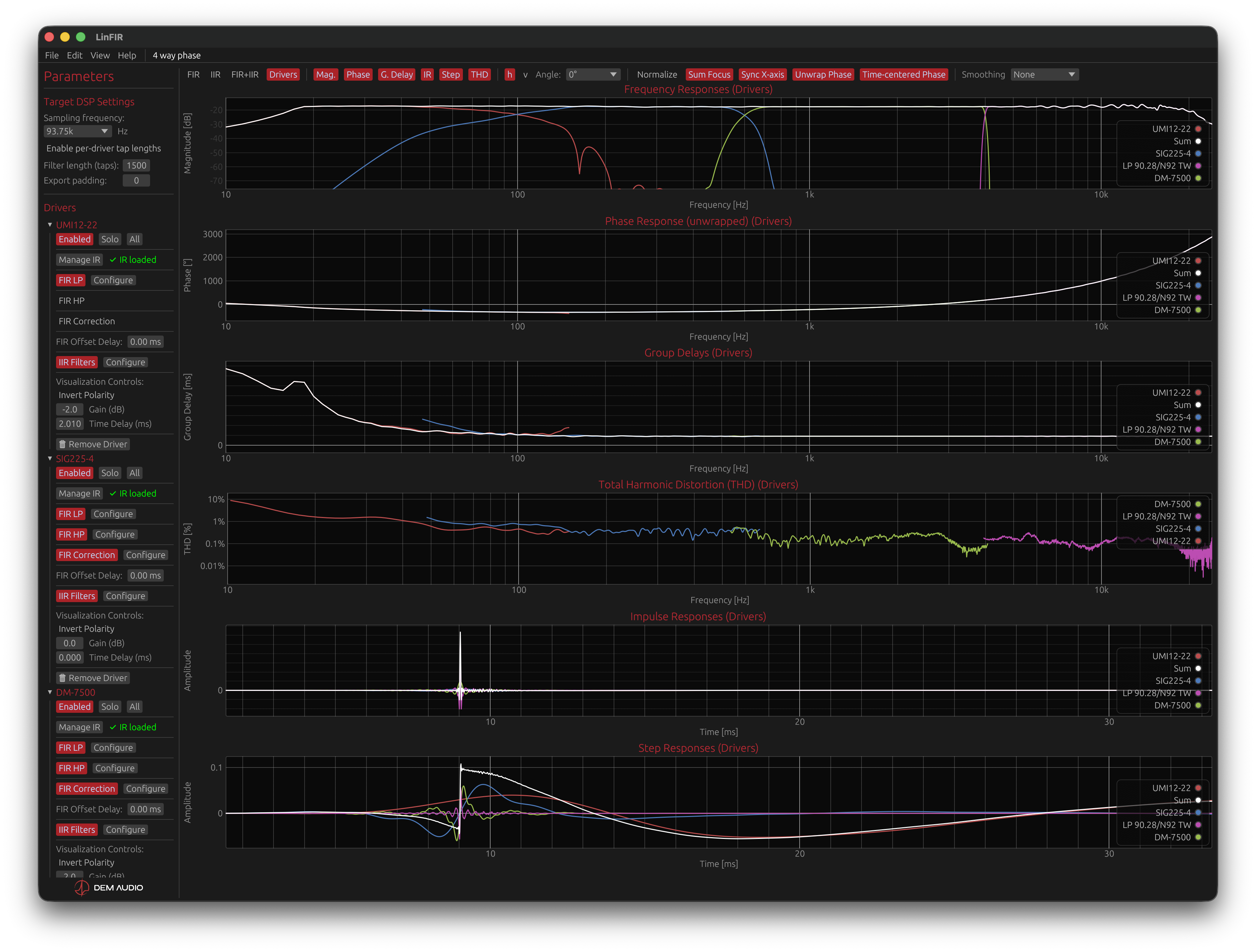
LinFIR offers three specialized operating modes, each designed for specific audio engineering workflows. The mode is selected during project creation and determines the available features and interface elements throughout the project’s lifetime.
Note on Hypex FusionAmp mode: The Hypex FusionAmp mode is a derivative of Loudspeaker Design mode. Everything documented for Loudspeaker Design — driver processing, crossover design, FIR/IIR filtering, measurement import, directivity analysis — applies equally to Hypex FusionAmp projects. The mode adds hardware-specific UI constraints (locked sample rate, fixed channel count, FIR tap limits, IIR biquad limit) that prevent invalid configurations and eliminate the need to manually track hardware limits during the design process.
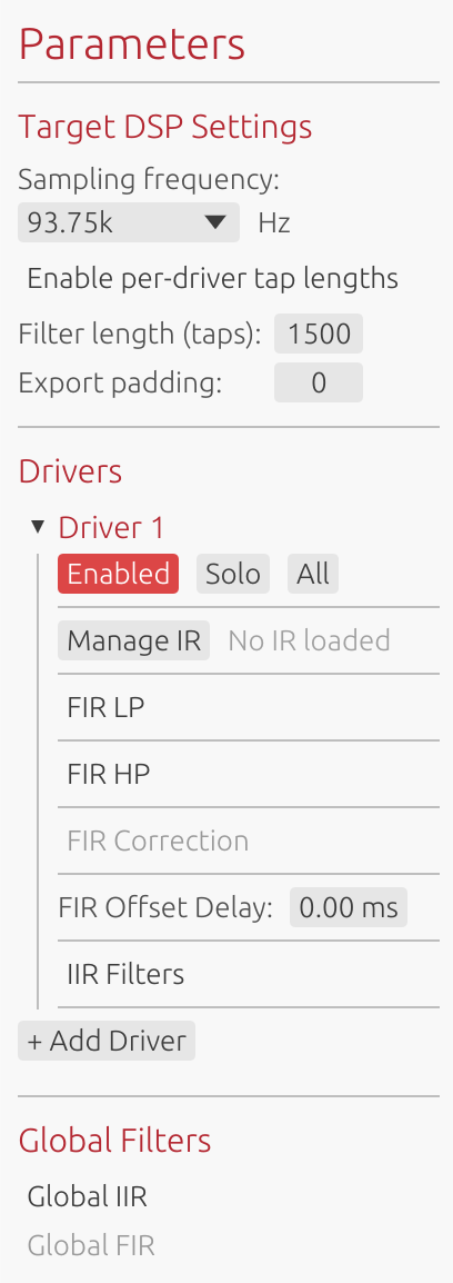
Loudspeaker Design Mode
Purpose
This mode is optimized for designing and analyzing multi-way loudspeaker systems. It provides comprehensive tools for crossover design, driver integration, and directivity analysis.
Key Features
- Multi-driver support: Design systems with multiple drivers (subwoofers, woofers, midranges, tweeters)
- Crossover: FIR and IIR crossover filters with various types
- Driver correction: Individual magnitude and phase correction for each driver
- Directivity tools: Analyze off-axis response and polar patterns (license required)
- Complete export: Export individual driver filters, global filters, and HFD configurations

Typical Workflow
- Create a new Loudspeaker Design project
- Import or measure impulse responses for each driver
- Design crossover filters (low-pass, high-pass)
- Apply frequency response corrections
- Analyze summed system response
- Export filters for DSP implementation
When to Use
- Designing passive loudspeaker conversions to active DSP
- Optimizing existing multi-way systems
- Analyzing driver interactions and phase relationships
- Creating custom crossover
- Performing anechoic or quasi-anechoic measurements
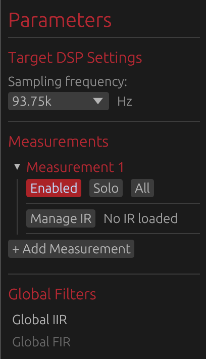
Room Calibration Mode
Purpose
Dedicated to in-room acoustic measurements and correction filter generation. This mode focuses on capturing multiple measurement positions, aligning them temporally, and creating averaged correction filters.
Key Features
- Multiple measurement positions: Capture IRs at different listening locations
- Automatic temporal alignment: GCC-PHAT algorithm aligns measurements
- Spatial averaging: Creates averaged response across measurement positions
- Global correction only: Simplified interface focused on room correction
- Streamlined export: Export only global correction filters
Typical Workflow
- Create a new Room Calibration project
- Configure sweep output channel
- Capture measurements at 3-5 different listening positions
- Measurements are automatically aligned using GCC-PHAT
- Design global correction filters (FIR and/or IIR)
- Export correction filters for room EQ implementation
UI Adaptations
When in Room Calibration mode, the interface adapts to focus on relevant features:
- Disabled: Directivity analysis tools (not applicable to room measurements)
- Simplified: Filter graphs show only global filters
- Restricted: Export options limited to global correction filters
- Hidden: Individual driver processing controls
Export Restrictions
Room Calibration projects export only:
- Global FIR correction filter (if enabled)
- Global IIR filters (Manual or Auto-EQ)
The following exports are disabled:
- HFD config export
- Detailed reports (TXT/PDF)
- Individual driver filters
This ensures clean, focused output for room correction workflows.
When to Use
- Correcting in-room frequency response
- Creating stereo-linked or mono room correction
- Working with existing loudspeaker systems
- Integrating with convolution engines
Hypex FusionAmp Mode
⚠️ License required: Creating Hypex FusionAmp projects requires a valid LinFIR license. See License for activation details.
Purpose
Hypex FusionAmp mode is a derivative of Loudspeaker Design mode tailored specifically for Hypex FusionAmp series amplifiers (FA122, FA123, FA251, FA252, FA253, FA501, FA502, FA503). All Loudspeaker Design features are available — driver processing, crossover design, FIR/IIR filtering, measurement import, directivity analysis — but several parameters are locked to match the DSP capabilities of the target hardware.
The goal is to eliminate manual bookkeeping: instead of counting biquads, tracking tap budgets, or checking compatibility after the fact, the UI enforces hardware limits in real time so the resulting configuration is always valid and ready to export.
Available Models
LinFIR supports all FusionAmp models:
- FA122: 2-channel amplifier (2 × 125W @ 4Ω)
- FA123: 3-channel amplifier (2 × 125W + 100W @ 4Ω)
- FA251: 1-channel amplifier (1 × 250W @ 4Ω)
- FA252: 2-channel amplifier (2 × 250W @ 4Ω)
- FA253: 2-channel amplifier (2 × 250W + 100W @ 4Ω)
- FA501: 1-channel amplifier (1 × 500W @ 4Ω)
- FA502: 2-channel amplifier (2 × 500W @ 4Ω)
- FA503: 3-channel amplifier (2 × 500W + 100W @ 4Ω)
Hardware Constraints
When in Hypex FusionAmp mode, several parameters are locked to match hardware specifications:
- Sample Rate: Fixed at 93.75 kHz (cannot be changed)
- Channel Count: Fixed by model (1, 2 or 3 channels, cannot add/remove drivers)
- IIR Filters: Maximum 15 biquads per channel
- FIR Filters: Fixed total tap count depends on FIR position (see below)
FIR Processing Modes
FusionAmp mode offers two mutually exclusive FIR processing configurations:
FIR IN (Input FIR)
Global FIR correction applied at the DSP input stage before channel processing.
- Location: Before IIR filters and channel routing
- Total taps: Fixed at 4500 (filter taps + padding)
- Use case: Global room correction, global speaker compensation
- Constraint: FIR Taps + Export padding = 4500 (always)
- UI behavior: Per-driver FIR controls are hidden; adjusting taps automatically adjusts padding to maintain 4500 total
FIR OUT (Output FIR)
FIR correction applied at the output stage, after IIR processing.
- Location: After IIR filters, per-channel or global
- Total taps: Fixed at 1500 per channel (filter taps + padding)
- Use case: Individual driver correction, per-channel equalization
- Constraint: Filter length (taps) + Export padding = 1500 (always, per driver or global)
- UI behavior: Adjusting taps automatically adjusts padding to maintain 1500 total
IIR Filter Constraints
FusionAmp DSP limits each channel to 15 biquads maximum. LinFIR enforces this through:
- Add Filter button: Automatically disabled when at 15 biquads
- Filter type restrictions: Types exceeding the limit are grayed out with tooltips
- Order limitations: Filter order sliders dynamically limited based on remaining capacity
- Auto EQ constraints: “Max Filters” parameter accounts for locked filters’ biquad usage
Note: For details on how biquad counts are calculated for different filter types, see the IIR Filtering section.
Key Features
- Hardware-matched UI: Interface adapts to show only applicable controls
- Automatic validation: Prevents configurations exceeding hardware limits
- Export compatibility: Direct HFD export for FusionAmp amplifiers
- Constraint warnings: Visual indicators when approaching limits
Typical Workflow
- Create new project: File → New Project → Hypex FusionAmp
- Select model (FA122, FA123, FA251, FA252, FA253, FA501, FA502, FA503)
- Choose FIR position (Input or Output)
- Import/measure impulse responses for each channel
- Design IIR filters (monitor biquad counter to stay within 15 biquad limit)
- Configure FIR correction (taps + padding always equals 4500 for IN or 1500 for OUT)
- Export HFD configuration file for amplifier
UI Adaptations
The interface automatically adjusts based on FIR position:
FIR IN mode:
- Global FIR section visible and active
- Per-driver FIR controls hidden
- Taps and padding controls linked to maintain 4500 total
- Adjusting taps automatically recalculates padding, and vice versa
FIR OUT mode with per-driver FIR:
- Per-driver FIR controls visible
- Each driver has linked taps/padding controls maintaining 1500 total
- Global FIR section hidden or disabled
FIR OUT mode without per-driver FIR:
- Taps and padding controls linked to maintain 1500 total
- Per-driver FIR controls hidden
Export Configuration
Hypex FusionAmp projects support:
- HFD export: Native configuration format for FusionAmp amplifiers
- FIR filter export: Individual channel FIR filters
- IIR filter export: Biquad coefficients per channel
When to Use
- Configuring Hypex FusionAmp series amplifiers
- Ensuring DSP configuration fits hardware constraints
- Exporting ready-to-use HFD configuration files
- Working within strict real-time processing limits
Limitations
⚠️ Hardware constraints cannot be bypassed:
- Sample rate is locked at 93.75 kHz
- Channel count is fixed by model (1, 2, or 3 channels)
- FIR total tap count is fixed (4500 for IN, 1500 for OUT) - taps and padding sum must always equal this value
- IIR biquad limit (15 per channel) is strictly enforced
- Cannot use both FIR IN and FIR OUT simultaneously
Mode Selection
Creating a New Project
Project mode is selected via File → New Project:
- Click “New Project”
- Choose between “Loudspeaker Design”, “Room Calibration”, or “Hypex FusionAmp”
- For Hypex FusionAmp: Select model (FA122/FA123/FA251/FA252/FA253/FA501/FA502/FA503) and FIR position (IN/OUT)
- For other modes: Configure initial project settings (sample rate, filter length, etc.)
- Begin working in the selected mode
Mode Permanence
⚠️ Important: Once a project is created, its mode cannot be changed. The mode is permanently associated with the project file.
To work in a different mode:
- Save your current project (if needed)
- Create a new project with the desired mode
- Import measurements or data as required
Choosing the Right Mode
Use Loudspeaker Design Mode when:
- Designing crossovers for multi-driver systems
- Analyzing individual driver characteristics
- Performing directivity analysis
- Working with anechoic or quasi-anechoic data
- Need flexible configuration options
Use Room Calibration Mode when:
- Correcting in-room frequency response
- Creating averaged room correction filters
- Working with existing complete loudspeaker systems
- Focusing on global system correction only
Use Hypex FusionAmp Mode when: (license required)
- Configuring Hypex FusionAmp series amplifiers
- Exporting HFD configuration files
- Need to ensure configurations match hardware limits (93.75 kHz, fixed taps, 15 biquads)
Best Practices
Room Calibration Mode
- Measurement count: Capture 3-5 measurements at different positions
- Position spacing: Keep positions within 30-50 cm of main listening area
- Height consistency: Use consistent microphone height across measurements
- Reference position: First measurement should be at primary listening position
- Correction philosophy: Apply gentle correction, avoid over-equalization
- Deep nulls: Don’t attempt to fill room mode nulls below 300 Hz
- Phase type: Consider minimum-phase FIR for reduced latency
- Acoustic treatment: Combine with room treatment for best results
Loudspeaker Design Mode
- Measurement quality: Use anechoic or quasi-anechoic measurements when possible
- Windowing: Gate reflections using IR time windowing
- Alignment: Align drivers using time delay controls, not FIR compensation delay
- Crossover design: Start with appropriate crossover frequencies and filter slopes
- Phase analysis: Monitor phase relationships between drivers
- Directivity: Capture multiple angles for comprehensive analysis (license required)
Mode Comparison Table
| Feature | Loudspeaker Design | Room Calibration | Hypex FusionAmp (license) |
|---|---|---|---|
| Multi-driver support | ✅ | ❌ (single “system”) | ✅ (1-3 fixed) |
| Individual driver filters | ✅ | ❌ | ✅ |
| Global filters | ✅ | ✅ | ✅ |
| Directivity analysis | ✅ (license) | ❌ | ✅ (license) |
| Multiple measurements | ✅ | ✅ | ✅ |
| Automatic alignment | ❌ | ✅ (GCC-PHAT) | ❌ |
| HFD export | ✅ | ❌ | ✅ |
| IIR filter export | ✅ | ✅ | ✅ (15 biquad limit) |
| Detailed reports | ✅ | ❌ | ✅ |
| THD analysis | ✅ | ❌ | ✅ |
| Sample rate | Configurable | Configurable | 93.75 kHz (locked) |
| Channel count | Configurable | 1 (mono/avg) | 1-3 (model-locked) |
| FIR total taps | Configurable | Configurable | Fixed: 4500 (IN) or 1500 (OUT) |
| IIR biquad limit | None | None | 15 per channel |
Hypex FusionAmp is a superset of Loudspeaker Design: all ✅ features from Loudspeaker Design are available, with the hardware constraints in the last rows added on top.
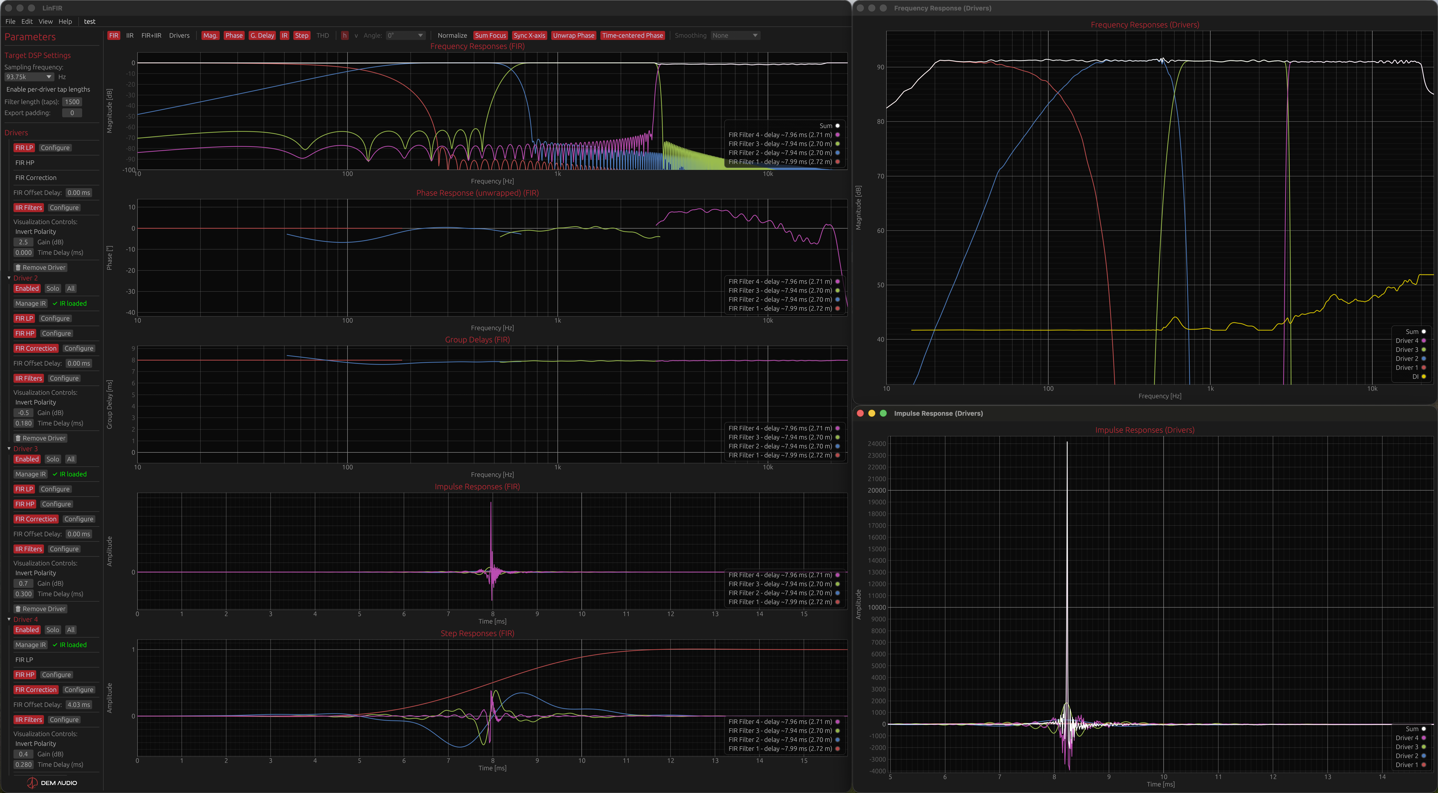
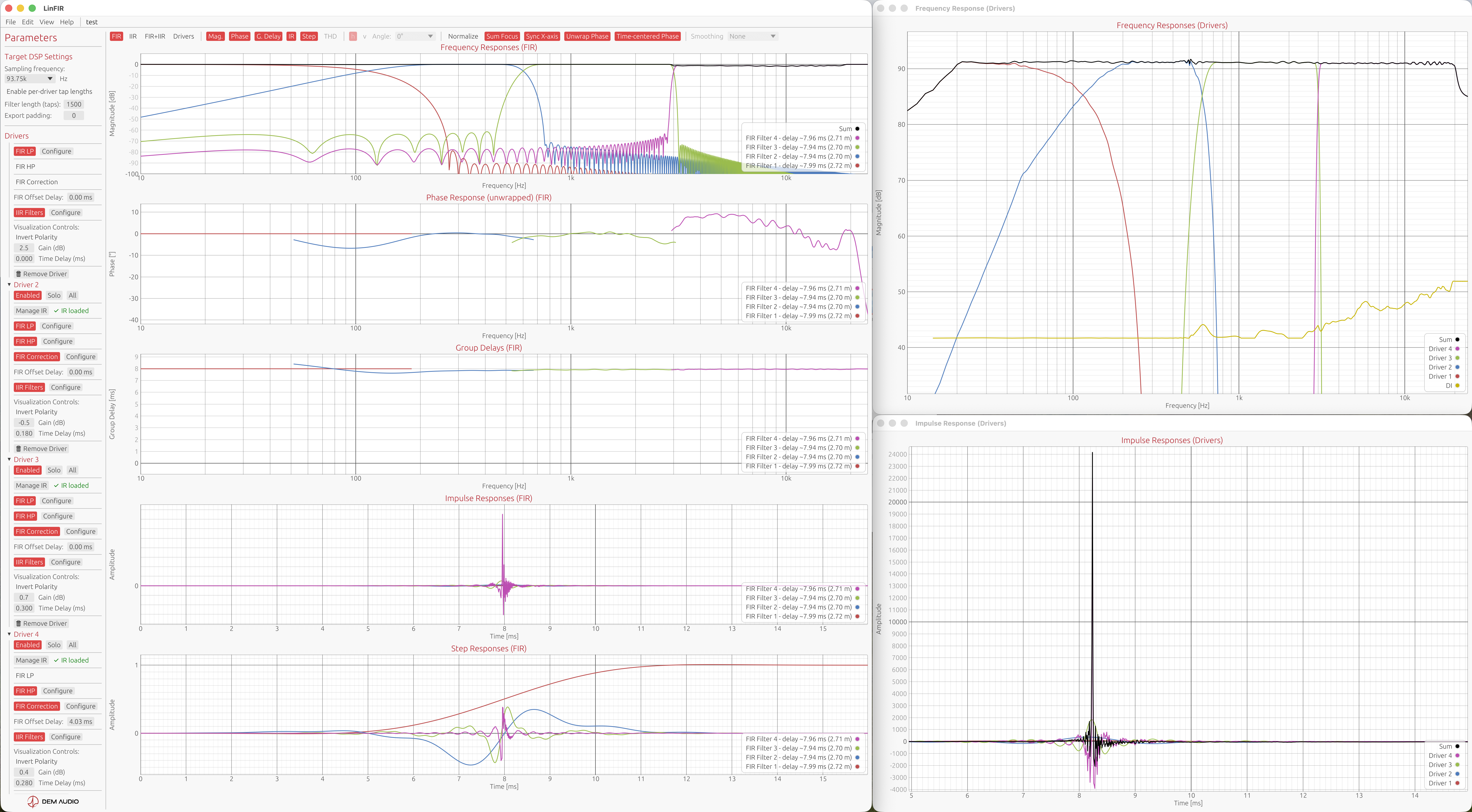
Graph Interaction & Display
This section covers all interactive features, display controls, and analysis tools available when working with LinFIR’s graphs.
Graph Toolbar
The graph toolbar provides comprehensive controls for selecting which data to display and how to visualize it. The toolbar adapts based on the project mode (Loudspeaker Design vs Room Calibration).
Loudspeaker Design Mode:


Room Calibration Mode:


Display Mode Selection
Purpose: Choose which stage of the signal processing chain to visualize.
Available modes:
- FIR - FIR filter responses only (crossovers, magnitude/phase correction)
- IIR - IIR filter responses only (parametric EQ, shelves, crossovers)
- FIR+IIR - Combined FIR and IIR responses
- Drivers (Loudspeaker Design) / Measurements (Room Calibration) - Full signal chain applied to driver or room measurements (theoretical system response)
Keyboard shortcuts:
- Press F to cycle through filter modes (FIR → IIR → FIR+IIR)
- Press D to switch to Drivers/Measurements mode
Mode behavior:
- Loudspeaker Design mode: Shows individual driver filters plus global filters
- Room Calibration mode: Shows only global filters in FIR/IIR/FIR+IIR modes
See Display Modes section below for detailed explanations of each mode.
Graph Visibility Toggles — “Graphs” Dropdown
Purpose: Show or hide specific graph types.
Graph types are grouped in the Graphs dropdown in the toolbar. Opening the dropdown reveals toggles for each graph type:
- Magnitude (M) - Frequency response in dB
- Impulse Response (I) - Impulse response in time domain
- Step Response (T) - Step response in time domain
- Group Delay (G) - Group delay in milliseconds
- Phase (P) - Phase response in degrees
- Harmonic Distortion (K) - (Loudspeaker Design / Hypex mode only)
Letters in parentheses indicate keyboard shortcuts. The dropdown stays open when toggling items, allowing multiple graphs to be shown or hidden without reopening it.
Note: Harmonic Distortion is only available in Loudspeaker Design / Hypex mode with Drivers display mode active, as harmonic distortion analysis is not applicable to in-room measurements.
License Feature: The HD graph displays the total harmonic distortion for all users. Individual harmonic curves (\(h_2\), \(h_3\), \(h_4\), \(h_5\)) are only available with a valid license.
Angle Selector (Loudspeaker Design / Hypex mode only)
Purpose: Select which off-axis measurement angle to display when drivers have directivity data.
- Horizontal angles: Typically ±15°, ±30°, ±45°, ±60°, ±75°, ±90°
- Vertical angles: Same as horizontal
- Toggle H/V: Switch between horizontal and vertical axis selection
Only available when at least one driver has off-axis measurements. The selector is hidden in Room Calibration mode as directivity analysis is specific to anechoic/quasi-anechoic loudspeaker measurements.
See Directivity Analysis for complete details on polar measurements and analysis.
Time Domain Options — “Time Domain” Dropdown
The Time Domain dropdown groups options that affect impulse and step response display.
Normalize
Purpose: Scale impulse and step responses to ±1 range for easier comparison.
When enabled:
- Impulse responses normalized to peak amplitude = 1
- Step responses normalized to maximum value = 1
- Useful for comparing relative timing and shape without amplitude differences
Focus on Summed Response
Purpose: Use the time boundaries of the summed impulse response for all IR and step response plots.
- Loudspeaker Design: All time-domain plots are framed around the summed driver output
- Individual curves remain visible within those boundaries
- Useful for evaluating overall system timing alignment
Phase Options — “Phase Options” Dropdown
The Phase Options dropdown is enabled only when the Phase graph is visible. It contains two options:
Unwrap Phase
Purpose: Display continuous phase response without ±180° wrapping discontinuities.
- Disabled: Phase wraps at ±180° (sawtooth pattern)
- Enabled: Phase continues beyond ±180° showing true accumulated phase shift
- Essential for analyzing linear phase filters and group delay
- Makes phase response easier to interpret across wide frequency ranges
Remove time of flight rotations
What is a time of flight? A pure propagation delay — the time it takes for sound to travel from the driver to the measurement microphone — appears in the phase response as a constant linear slope: the further the impulse response peak is from t = 0, the steeper the slope, and the more the phase accumulates rotations across the frequency range. This linear ramp carries no useful information about the filter or driver behaviour; it just reflects the physical distance between source and mic.
This option removes that linear component, leaving only the non-linear phase rotations introduced by the filters and the acoustics of each driver. The result is a much flatter, easier-to-read phase curve, and — when multiple drivers are shown — it becomes straightforward to compare their phase alignment without the bulk delay dominating the picture.
- Disabled: Phase includes the full linear delay component (steep slope proportional to time of flight)
- Enabled: Linear component subtracted, phase flattens around 0° — non-linear deviations stand out clearly
HD Display Mode (Loudspeaker Design mode only)
Purpose: Select how harmonic distortion values are displayed on the HD plot.
Available display modes:
- Percent (%) - Traditional percentage representation
- dB (relative) - Relative level compared to fundamental
- dB (absolute) - Absolute RMS level of harmonics
Percent (%) Mode:
Displays harmonic distortion as a percentage relative to the fundamental (\(h_1\)). Values above 100% are possible when harmonic components exceed the fundamental level (e.g., below the driver’s resonance frequency).
dB (relative) Mode:
Expresses harmonic distortion relative to the fundamental (\(h_1\)) in decibels. Negative values indicate harmonics are quieter than the fundamental; positive values indicate harmonics exceed the fundamental. For example:
- -40 dB ≈ 1% distortion
- -60 dB ≈ 0.1% distortion
- -80 dB ≈ 0.01% distortion
- 0 dB = 100% distortion (harmonics equal the fundamental)
Useful for evaluating signal-to-distortion ratio.
dB (absolute) Mode:
Shows the absolute level of the harmonics alone, without normalization. This mode is useful for comparing distortion levels across different SPL measurements, as it shows the actual acoustic power in harmonic components regardless of the fundamental level.
Individual Harmonics:
All three modes also display individual harmonic curves (\(h_2\), \(h_3\), \(h_4\), \(h_5\)) with dashed/dotted line styles. The selected mode applies to both the total HD curve and individual harmonics.
License Feature: Individual harmonic curves (\(h_2\)-\(h_5\)) are only available with a valid license.
Smoothing
Purpose: Apply smoothing to magnitude, HD, directivity, group delay and phase plots.
Smoothing options:
- None - No smoothing (raw response)
- 1/48 octave - Very fine smoothing
- 1/24 octave - Fine smoothing
- 1/12 octave - Moderate smoothing
- 1/6 octave - Coarse smoothing
- 1/3 octave - Very coarse smoothing
- ERB - Perceptually-motivated variable smoothing (see below)
Applies to:
- Magnitude (frequency response)
- Group delay
- Phase (preserves driver alignment via trend removal method)
- HD (Harmonic Distortion)
- Directivity Analysis (sonogram)
Does not affect: Time-domain plots (impulse, step response)
ERB Smoothing:
ERB (Equivalent Rectangular Bandwidth) smoothing uses a variable bandwidth that corresponds to the frequency resolution of the human auditory system. The smoothing bandwidth follows the formula: (107.77f + 24.673) Hz, where f is frequency in kHz.
This results in:
- Heavy smoothing at low frequencies (~1 octave at 50Hz, 1/2 octave at 100Hz, 1/3 octave at 200Hz)
- Moderate smoothing at mid frequencies (approximately 1/6 octave above 1kHz)
- Natural perceptual weighting that reflects how the ear integrates frequency information
ERB smoothing is particularly useful for:
- Understanding what a listener actually perceives
- Comparing measurements to subjective listening impressions
- Evaluating whether fine response details are audible
Note: Smoothing is cosmetic and does not affect filter calculations or exports. See Fractional Octave Smoothing section below for detailed behavior.
Mouse & Trackpad Controls
Zoom Controls
Zoom In - Multiple methods:
- Box zoom: Right-click and drag to select a region
- Trackpad pinch: Pinch gesture to zoom in/out
- Mouse wheel: Scroll to move the view within a graph
Zoom Out:
- Double-click anywhere on a graph to reset to auto-calculated bounds
- Double-click re-enables auto-bounds mode (graphs automatically adjust to data range)
Pan
Left-click and drag to move the view within a zoomed graph.
Legend Interaction
Click on color dots in the legend to show/hide individual curves:
- Hidden curves are grayed out in the legend
- Click again to show the curve
- Useful for isolating specific drivers or filters
Detach Graphs
Right-click on any graph to open it in a separate window:
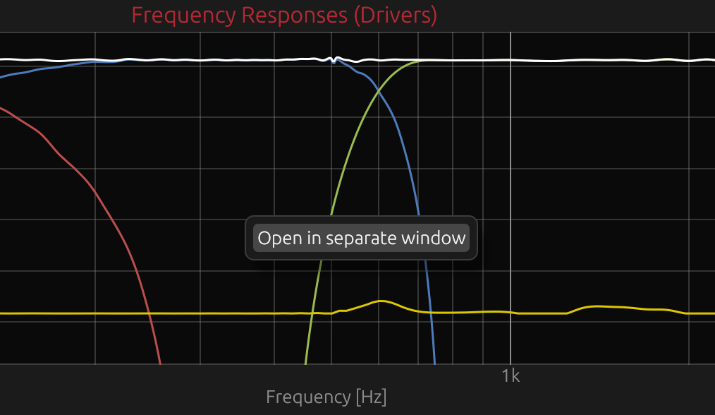
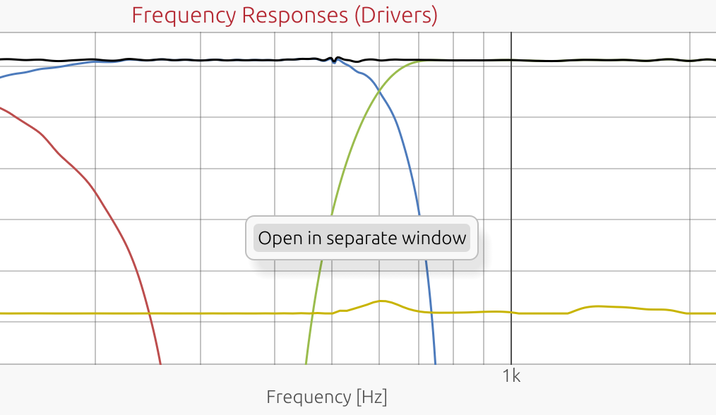
- All graph types supported (Frequency, Phase, Group Delay, Impulse, Step, HD)
- Detached windows render in real-time following the active display mode
- Multiple graphs can be opened simultaneously for side-by-side comparison
- Ideal for multi-monitor setups and detailed analysis workflows
- Close detached windows: Cmd+W (macOS) / Ctrl+W (Windows)
Display Modes
Project Mode Impact
LinFIR supports two project modes that affect display terminology:
- Loudspeaker Design - Speaker design with drivers
- Room Calibration - Multi-position measurements for room correction
In Room Calibration mode:
- “Drivers” mode is renamed to “Measurements”
- Individual measurement curves are shown in Measurements mode
- Filter modes (FIR/IIR/FIR+IIR) display only global filters
In Loudspeaker Design mode:
- “Drivers” mode displays individual drivers
- Filter modes show both per-driver filters and global filters
Filters vs. Drivers/Measurements Mode
Filters Mode (Keyboard: F):
- Shows individual filter responses (FIR, IIR, or FIR+IIR combined)
- Press F multiple times to cycle through filter submodes:
- FIR Filters - Shows only FIR filter responses
- IIR Filters - Shows only IIR filter responses
- FIR+IIR Filters - Shows combined FIR and IIR responses
- Loudspeaker Design: Per-driver crossover and correction filters displayed separately
- Room Calibration: Only global filters are shown
- Global filters shown as additional curves
- Useful for analyzing filter design and frequency response shaping
Drivers/Measurements Mode (Keyboard: D):
- Loudspeaker Design: Shows combined driver + filter responses (acoustic output)
- Each curve represents the complete signal chain for that driver
- Sum curve shows the total system response at listening position
- Room Calibration: Shows individual measurement positions and averaged response
- Each curve represents a raw measurement location (no filters applied)
- Sum curve shows the averaged response with global filters applied
- Useful for analyzing final acoustic performance
Graph Visibility Toggles
Show/hide individual graph types using keyboard shortcuts:
- M - Toggle Magnitude (Frequency Response) plot
- P - Toggle Phase Response plot
- G - Toggle Group Delay plot
- I - Toggle Impulse Response plot
- T - Toggle Step Response plot
- K - Toggle HD (Harmonic Distortion) plot
X-Axis Synchronization
Toggle: X key or toolbar button
When enabled, Sync X-axis synchronizes the horizontal axis across related plots:
Frequency Plots (Magnitude, Phase, Group Delay, Directivity Analysis):
- All plots share the same frequency range
- Zooming any plot updates all frequency plots simultaneously
- Double-click resets all frequency plots to full range
Time Plots (Impulse, Step Response):
- All time-domain plots share the same time range
- Zooming any plot updates all time plots simultaneously
- Double-click resets all time plots to full range
Independent Y-Axes:
- Each plot maintains its own vertical scale
- Y-axis auto-bounds independently for each graph type
Use Cases:
- Compare magnitude and phase behavior at the same frequency
- Analyze impulse and step response in the same time window
- Maintain consistent zoom across multiple graph types
Impulse & Step Response Normalization
Toggle: N key or toolbar button
Normalizes impulse and step responses to peak amplitude = 1.0:
Purpose:
- Allows visual comparison between responses with different amplitudes
- Focuses on filter shape and time-domain characteristics
- Eliminates gain differences for easier visual analysis
Effect:
- All IR and SR curves are scaled to the same peak height
- Does not affect magnitude or phase plots
- Purely visual - does not modify underlying data
Use Cases:
- Compare filter shapes between drivers with different sensitivity
- Analyze time-domain behavior without gain differences obscuring details
- Identify pre-ringing or timing issues across multiple drivers
Focus on Summed Response
Toggle: S key or Time Domain dropdown (Drivers/Measurements mode only)
Synchronizes the time window of all temporal plots (Impulse & Step Response) to the Sum/Average curve boundaries:
How it Works:
- Analyzes the Sum/Average impulse response to find its energy boundaries
- Detects first and last samples above -60 dB threshold (1/1000th of peak)
- Adds configurable margins before and after the detected energy region
- Applies the same time window to all temporal plots (both Impulse and Step Response)
- Enables auto-bounds for all time plots
Behavior:
- Requires at least 2 active curves to activate (otherwise ignored)
- Focuses all temporal plots on the main acoustic energy of the Sum/Average response
- Individual driver/measurement curves are zoomed to the same time window as the sum
- Easier to compare arrival times and transient behavior across all curves
- Works with adaptive display mode margins (configurable in Settings)
Use Cases:
- Loudspeaker Design: Quickly identify timing alignment issues across drivers
- See if all drivers arrive within the sum’s main energy window
- Detect delays or misalignment relative to system response
- Room Calibration: Focus on the averaged room response energy region
- Compare individual measurement positions to the average response timing
- Identify room reflections within the main energy window
- Eliminate clutter from pre-ringing or tail noise outside the main energy region
Only available in Drivers/Measurements Mode (not applicable to individual filters).
Note: Works in both Loudspeaker Design and Room Calibration project modes when display mode is set to Drivers/Measurements.
Phase Display Options
Unwrap Phase
Toggle: U key or toolbar button
Controls phase display format:
Wrapped Phase (default):
- Phase values constrained to ±180°
- Shows discontinuities (phase wraps) at ±180° boundaries
- Easier to read for simple filters
- Standard display format for most audio applications
Unwrapped Phase:
- Continuous phase values extending beyond ±180°
- Shows total accumulated phase shift
- Useful for analyzing group delay trends and overall phase shift
Note: Group delay is always computed from unwrapped phase internally. The Unwrap toggle only affects phase display, not group delay accuracy.
Remove time of flight rotations
Toggle: C key or Phase Options dropdown (next to Unwrap Phase)
A pure propagation delay translates into a linear slope in the phase response — the further the impulse response peak is from t = 0, the steeper the slope, and the more rotations accumulate across the frequency range. This linear ramp is entirely determined by the physical distance between the driver and the microphone and does not reveal anything about filter behaviour or driver characteristics.
This option removes that linear component via a linear regression on the IR peak position, leaving only the non-linear phase introduced by the filters and acoustics. Phase curves become much flatter, easier to read, and directly comparable across drivers regardless of their physical placement.
Removes the linear phase component (constant group delay) from phase responses:
Algorithm:
- Computes linear phase slope from IR peak position for all curves (drivers and filters)
- Subtracts the constant group delay (linear phase shift)
- Flattens phase around 0° while preserving relative phase differences
- Works with both wrapped and unwrapped phase display modes
In Loudspeaker Design Mode (Drivers):
When multiple speakers are active:
- Removes the linear delay of the Sum curve from all responses
- Centers all driver phases around 0° relative to the system response
- Highlights phase alignment issues between drivers
- Makes phase differences visible without bulk delay obscuring them
When single driver is active:
- Removes the linear component of that driver’s phase
- Flattens phase around 0° to show only non-linear phase shifts
In Room Calibration Mode (Measurements):
- Independent correction: Removes the linear phase component of each individual measurement independently
- No shared reference - each measurement position is treated separately
- Flattens each measurement’s phase around 0°
- Useful for comparing phase behavior across different room positions without timing offsets
- The averaged curve also has its own linear component removed
In Filters Mode (FIR, IIR, FIR+IIR):
- Per-filter correction: Removes the linear phase component of each individual filter
- Flattens each filter’s phase around 0°
- Reveals only non-linear phase rotations introduced by the filter
- Useful for analyzing filter phase behavior independent of bulk delay
Use Cases:
- Identify phase alignment issues between drivers without delay obscuring differences
- Visualize phase rotations introduced by filters (independent of linear delay)
- Compare filter phase characteristics across different designs
- Verify minimum-phase vs. linear-phase behavior
Fractional Octave Smoothing
Control: Dropdown menu in toolbar (None, 1/48 oct to 1/3 oct, or ERB)
Apply smoothing to reduce measurement noise and reveal trends:
Fixed Fractional-Octave Smoothing:
- No smoothing - Show raw response (no averaging)
- 1/48 octave - Very fine smoothing (highest detail)
- 1/24 octave - Fine smoothing
- 1/12 octave - Moderate smoothing (default)
- 1/6 octave - Coarse smoothing
- 1/3 octave - Very coarse smoothing (lowest detail)
ERB (Equivalent Rectangular Bandwidth) Smoothing:
ERB smoothing uses a frequency-dependent bandwidth that models the human auditory system’s frequency resolution. Unlike fixed fractional-octave smoothing, ERB adapts its bandwidth at each frequency according to psychoacoustic research.
Bandwidth formula: (107.77f + 24.673) Hz, where f is in kHz
Frequency-dependent behavior:
- 50 Hz → ~1 octave bandwidth (heavy smoothing)
- 100 Hz → ~1/2 octave bandwidth
- 200 Hz → ~1/3 octave bandwidth
- 1 kHz and above → ~1/6 octave bandwidth (leveling out)
When to use ERB smoothing:
- To see what the ear actually perceives (perceptually accurate)
- When evaluating audibility of response features
- To match listening test results with measured data
- For publication-quality graphs that reflect human hearing
When to use fixed fractional-octave smoothing:
- For equalization and correction work (1/6 or 1/12 octave recommended)
- When analyzing crossover behavior in detail
- To maintain consistent resolution across all frequencies
- For technical comparisons between drivers
Effect:
- Wider smoothing = smoother curves, less detail
- Narrower smoothing = more detail, more noise visible
- ERB = perceptually-weighted smoothing (variable with frequency)
Applies to:
- Frequency response (magnitude), HD, Directivity Analysis (sonogram), group delay and phase plots
- Does not affect time-domain plots (impulse responses)
Note: Smoothing is applied after all processing (filters, crossovers, correction). It affects display only, not exported data. It can also alter crossover slopes on the graphs.
Impulse Response Analysis
Automatic Pre-Ringing Detection
When hovering over impulse response curves, LinFIR displays additional analysis information:
Pre-ring Level (in dB relative to peak):
- Weighted RMS measurement of signal energy before the main peak
- Analysis stops at the last zero-crossing before peak (excludes rising edge)
- Uses Hilbert envelope to capture perceptible energy regardless of phase
- Perceptually weighted: energy closer to the peak is less penalized (temporal masking)
- Displayed as:
Pre-ring: -50.0 dB (Likely masked)
Algorithm Details:
- Find the impulse peak position and amplitude
- Find the last zero-crossing before the peak (to exclude the rising edge)
- Extract the pre-ringing region (from start to zero-crossing)
- Calculate the Hilbert envelope of the pre-ringing region
- Apply sigmoid weighting (closer to peak = less perceptual penalty)
- Masking time at 50% penalty: 0.6 ms (default)
- Weight floor: 0.2 (minimum weight for distant pre-ring)
- Weight ceiling: 1.0 (maximum weight for near-peak pre-ring)
- Calculate weighted RMS of the envelope
- Convert to dB relative to peak amplitude
Weighting Rationale:
- Pre-ringing close to the peak is masked by the main transient (temporal masking)
- Pre-ringing far from the peak is more audible (less masking)
- Sigmoid function models gradual transition from masked to unmasked
Risk Assessment Labels
Pre-ringing levels are classified based on typical perceptual thresholds (indicative):
| Level (dB) | Risk Assessment | Description |
|---|---|---|
| ≤ -36 dB | Likely masked | Generally inaudible, masked by main transient |
| -36 to -24 dB | Low risk | May be perceptible in some cases (quiet passages) |
| -24 to -12 dB | Moderate risk | Likely perceptible depending on program material |
| > -12 dB | High risk | Potentially objectionable, consider reducing filter length |
Important Notes:
- These are indicative estimates, not absolute rules
- Actual audibility depends on:
- Program material (transient-rich vs. sustained tones)
- Listening level
- Individual hearing sensitivity
- Room acoustics and background noise
- Use as a guideline for filter design, not strict limits
- Shorter FIR filters or increased causality reduce pre-ringing at the cost of magnitude and phase accuracy
Trade-offs:
- Longer FIR filters → More pre-ringing, better magnitude/phase accuracy
- Shorter FIR filters → Less pre-ringing, reduced correction capability
- Higher causality (e.g., minimum-phase) → Less pre-ringing, potential phase distortion
- Linear-phase (causality = 0) → Maximum pre-ringing, linear phase
Auto-Bounds Behavior
LinFIR automatically adjusts graph bounds to fit data:
Auto-Bounds Enabled (default):
- Graphs automatically scale to show all data
- Y-axis adjusts when switching between drivers or display modes
- X-axis adjusts based on data range (frequency or time)
Auto-Bounds Disabled (after user interaction):
- Manual zoom/pan disables auto-bounds for that axis
- Graph retains user-specified bounds
- Switching modes preserves manual bounds
- Double-click re-enables auto-bounds and resets to calculated range
Per-Axis Independence:
- X-axis and Y-axis auto-bounds are independent
- Dragging vertically disables Y auto-bounds, preserves X auto-bounds
- Dragging horizontally disables X auto-bounds, preserves Y auto-bounds
- Box zoom (right-click drag) disables both X and Y auto-bounds
Per-Graph Independence:
- Each graph type has independent auto-bounds state
- Zooming Frequency plot does not affect Impulse plot
- Switching between display modes preserves per-graph bounds
Keyboard Shortcuts Summary
Display Modes
- F - Switch to Filters display mode
- D - Switch to Drivers/Measurements display mode
Display Controls
- X - Toggle X-axis synchronization
- N - Toggle normalize impulse and step responses
- U - Toggle unwrap/wrap phase response
- C - Toggle time of flight rotation removal
- S - Toggle focus on summed impulse response (Drivers/Measurements mode only)
- R - Toggle Directivity Analysis window (Loudspeaker Design mode only, requires license)
Graph Visibility
- M - Toggle Magnitude Response plot
- P - Toggle Phase Response plot
- G - Toggle Group Delay plot
- I - Toggle Impulse Response plot
- T - Toggle Step Response plot
- K - Toggle HD (Harmonic Distortion) plot
Related Documentation
- Settings - Graph resolution, titles, colors
- Keyboard Shortcuts - Complete shortcut reference
- Driver Processing - Filters affecting graph display
- System Processing - Global filters and sum calculation
Keyboard Shortcuts
This is a comprehensive reference of all keyboard shortcuts available in LinFIR.
Note: On macOS, use Cmd (⌘). On Windows/Linux, use Ctrl.
File Operations
| Shortcut | Action | Description |
|---|---|---|
| Cmd+S / Ctrl+S | Save Project | Saves the current project to disk. If no file path exists, prompts for location (Save As). |
| Cmd+E / Ctrl+E | Export Project | Opens file dialog to export project as a new .lnf file (Save As). |
Context:
- Works in main window and all detached windows
- Disabled when text input fields have focus (to avoid conflicts)
- Auto-save runs every 60 seconds in the background (if enabled)
Window Operations
| Shortcut | Action | Description |
|---|---|---|
| Cmd+, / Ctrl+, | Open Settings | Opens the Settings window. If already open, brings it to front. |
| Cmd+W / Ctrl+W | Close Window | Closes the currently focused window (detached graphs, dialogs, etc.). Does not close main window. |
| H | Toggle Documentation | Opens/closes the embedded documentation browser (localhost:3030). |
Context:
- Cmd+W works in detached graph windows, driver IR windows, HFD export window, etc.
- Cmd+, is a system-wide shortcut to access application settings
- H toggles documentation visibility globally
Display Modes
| Shortcut | Action | Description |
|---|---|---|
| D | Drivers Mode | Switches to Drivers display mode (combined driver + filter responses). |
| F | Filters Mode | Cycles through filter display modes: FIR → IIR → FIR+IIR → FIR. |
Behavior:
- D: Shows acoustic output (driver impulse + all filters applied)
- F: Shows individual filter responses
- First press: FIR filters only
- Second press: IIR filters only
- Third press: FIR+IIR combined
- Fourth press: Back to FIR filters
Context: Only active when no text input has focus.
Display Controls
| Shortcut | Action | Description |
|---|---|---|
| X | Sync X-Axis | Toggles X-axis synchronization across related plots (frequency plots and time plots). |
| N | Normalize IR/SR | Normalizes impulse and step responses to peak amplitude = 1.0 for visual comparison. |
| U | Unwrap Phase | Toggles between wrapped (±180°) and unwrapped (continuous) phase display. |
| C | Remove time of flight rotations | Removes linear phase component (constant group delay) from phase responses. |
| S | Focus on Summed Response | Focuses all time-domain plots on the boundaries of the summed impulse response (Drivers mode only). |
Details:
-
X (Sync X-Axis):
- Frequency plots (Magnitude, Phase, Group Delay) share X-axis
- Time plots (Impulse, Step) share X-axis
- Y-axes remain independent
-
N (Normalize):
- Visual only - does not affect exported data
- Useful for comparing filter shapes with different gains
-
U (Unwrap Phase):
- Wrapped: phase constrained to ±180° (discontinuities)
- Unwrapped: continuous phase beyond ±180° (smooth)
-
C (Remove time of flight rotations):
- Removes linear phase (constant group delay) via linear regression
- Flattens phase around 0° to show only non-linear behavior
- In Drivers mode: removes Sum curve delay from all responses
- In Filters mode: per-filter linear phase removal
-
S (Focus on Summed Response):
- Only available in Drivers mode
- Calculates time boundaries from summed impulse
- Auto-enables auto-bounds for all time plots
Context: Only active when no text input has focus.
Graph Visibility Toggles
| Shortcut | Action | Description |
|---|---|---|
| M | Toggle Magnitude | Shows/hides frequency response (magnitude) plot. |
| P | Toggle Phase | Shows/hides phase response plot. |
| G | Toggle Group Delay | Shows/hides group delay plot. |
| I | Toggle Impulse | Shows/hides impulse response plot. |
| T | Toggle Step | Shows/hides step response plot. |
| K | Toggle Harmonic Distortion | Shows/hides Harmonic Distortion plot. |
Behavior:
- Each toggle is independent
- State persists across sessions (saved in project)
Context: Only active when no text input has focus.
Advanced Features
| Shortcut | Action | Description |
|---|---|---|
| R | Toggle Directivity Analysis | Opens/closes directivity analysis window (Loudspeaker Design mode only, valid license required). |
| W | Toggle Spectrogram | Opens/closes the Spectrogram window (valid license required). |
| J | Toggle Distortion IR | Opens/closes the Distortion Impulse Responses window (Loudspeaker Design mode only, valid license required). |
Requirements:
- R and J only work in Loudspeaker Design and Hypex FusionAmp modes (not Room Calibration)
- R, W, and J require a valid license
Context: Only active when no text input has focus.
Undo/Redo
| Shortcut | Action | Description |
|---|---|---|
| Cmd+Z / Ctrl+Z | Undo | Reverts the last change (filter, gain, delay, etc.). |
| Cmd+Shift+Z / Ctrl+Shift+Z | Redo | Re-applies the last undone change. |
Behavior:
- Full project state snapshots
- Limited undo history to 10 snapshots (constrained by memory)
- Works in main window and all viewport windows (Driver IR, HFD export, etc.)
Context: Disabled when text input fields have focus.
Dialog-Specific Shortcuts
Shortcut Contexts
LinFIR disables shortcuts based on context to avoid conflicts:
When Text Input Has Focus
The following shortcuts are disabled when typing in text fields (IR names, filter frequencies, etc.):
- All single-letter shortcuts (D, F, J, M, K, G, I, T, P, U, C, X, S, N, R, W, H)
- Undo/Redo (Cmd+Z, Cmd+Shift+Z)
- Save/Export (Cmd+S, Cmd+E)
- Settings (Cmd+,)
Still active:
- Close window (Cmd+W)
When Any Input Window is Open
Certain shortcuts are disabled when modal dialogs or input windows are open:
- Save (Cmd+S)
- Export (Cmd+E)
This prevents accidental saves while configuring settings or importing files.
Platform-Specific Notes
macOS
- Use Cmd (⌘) for all modifier shortcuts
- Cmd+W closes windows but not the main application window
- Cmd+Q quits the application (system shortcut)
- Cmd+, is the standard macOS shortcut for Preferences/Settings
Windows/Linux
- Use Ctrl for all modifier shortcuts
- Ctrl+W closes windows
- Alt+F4 quits the application (system shortcut)
Quick Reference Card
File
- Cmd+S - Save
- Cmd+E - Export Project
Window
- Cmd+W - Close Window
- Cmd+, - Settings
- H - Documentation
Display
- D - Drivers Mode
- F - Cycle Filters Mode
- X - Sync X-Axis
- N - Normalize IR/SR
- U - Unwrap Phase
- C - Remove time of flight rotations
- S - Focus on Summed Response
Graphs
- M - Magnitude
- P - Phase
- G - Group Delay
- I - Impulse
- T - Step
- K - Harmonic Distortion
Advanced
- R - Directivity Analysis (license required)
- W - Spectrogram (license required)
Edit
- Cmd+Z - Undo
- Cmd+Shift+Z - Redo
Related Documentation
- Graph Interaction - Mouse controls, zoom, pan, detach graphs
- Settings - Configure default display modes and preferences
- Driver Processing - Filter controls affected by shortcuts
- System Processing - Global filters and display modes
- Directivity Analysis - Directivity Analysis window (R key)
- Spectrogram - Spectrogram window (W key)
General Settings
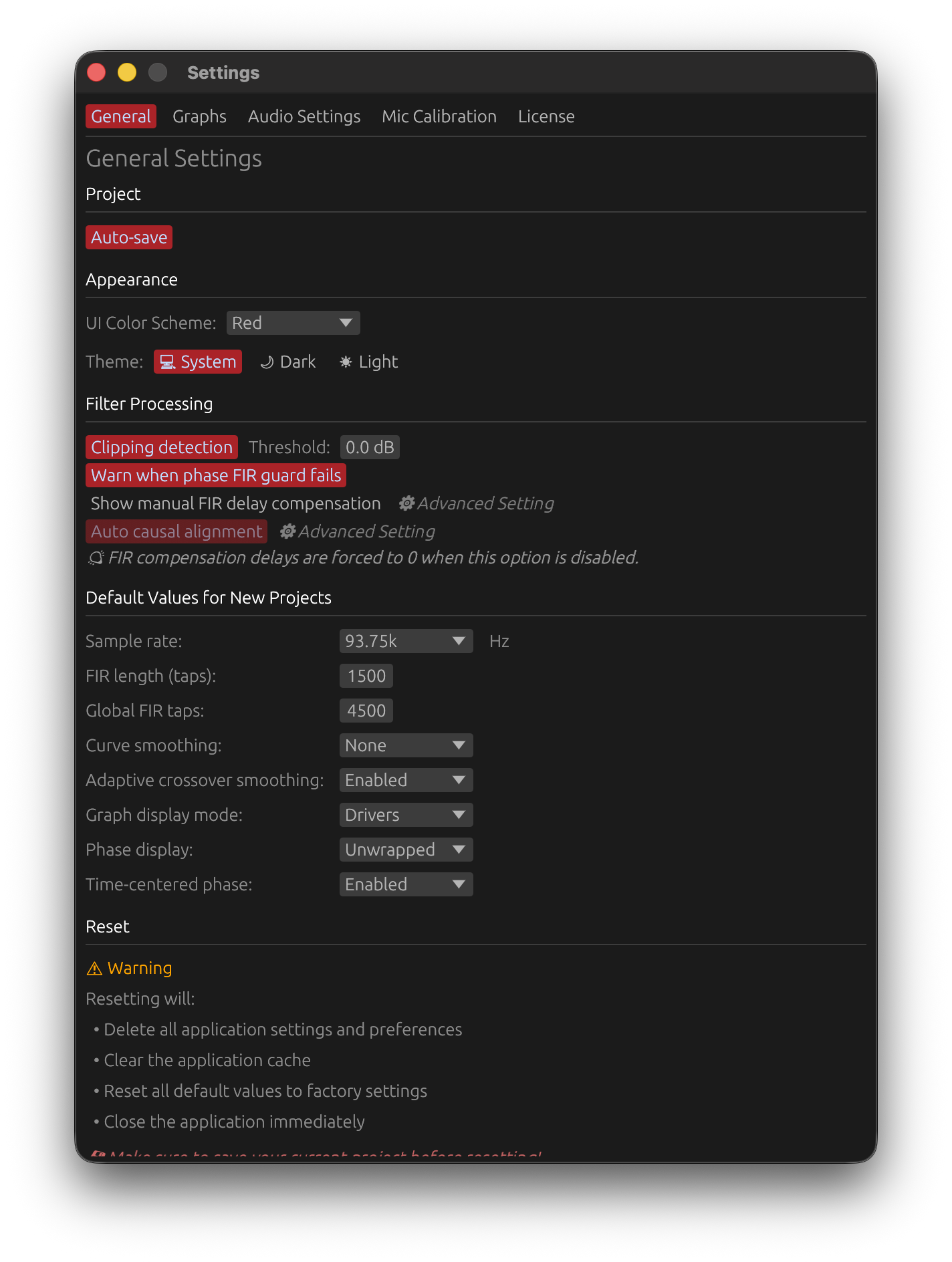
Appearance
Customize the visual appearance of the LinFIR interface.
UI Color Scheme
Choose between two color themes for LinFIR’s interface elements:
- Red (default): Custom red accent colors for headers, titles, and active buttons
- Blue: Standard egui theme with blue accents
What changes:
- Section headers (Parameters, Drivers, Global Filters)
- Graph titles (Frequency Responses, Impulse Responses, etc.)
- Active button colors and selection highlights
- Accent colors throughout the interface
Application: Changes apply immediately without requiring restart.
Theme (Light/Dark Mode)
Switch between light mode and dark mode using the system theme preference buttons.
- Light mode: Bright background, dark text
- Dark mode: Dark background, light text
- Follow system: Automatically matches your operating system theme preference
Filter Processing
Settings that affect how filters are computed and validated.
Clipping Detection
Default: Enabled
Threshold: 0 dB (configurable from −5 to +2 dB)
When enabled, LinFIR analyzes filter chains to detect potential clipping and suggests gain adjustments.
How it works:
- Generates a deterministic periodic pink-noise test signal covering 20 Hz to 20 kHz
- Spectral slope: −3 dB/octave (represents typical programme material)
- Band-shaped: 12 dB/oct high-pass at 20 Hz, 24 dB/oct low-pass at 20 kHz
- RMS ≈ −24 dBFS, peak = −6 dBFS (crest factor ≈ 12 dB)
- Applies all active filters to the test signal
- Warns when filter output exceeds the configured threshold
- Suggests gain reduction to bring peak below 0.95 × threshold (leaving a small safety margin)
Threshold setting: The threshold controls the detection sensitivity relative to digital full scale (0 dBFS):
- 0 dB (default): warn when the filter output reaches or exceeds full scale — the standard safety level
- Negative values (−1 to −5 dB): conservative — trigger the warning before reaching full scale, leaving extra headroom.
- Positive values (+1, +2 dB): lenient — only warn when the output is significantly above full scale. Use with caution: values above 0 dB allow actual clipping to go unreported
⚠️ Setting the threshold above 0 dB means clipping can occur without any warning.
Important clarifications:
⚠️ Measurement levels are not tested - Clipping warnings are purely about filter processing, not your imported measurements. The test signal is synthetic and independent of measurement amplitude.
⚠️ Phase processing can cause clipping even with flat magnitude responses - Filters with visually reasonable frequency responses can produce temporal peaks exceeding 0 dBFS. This is especially common with:
- Phase correction filters combined with other filters (without crossovers)
- All-pass filters that only modify phase
- Multiple FIR filters with different causality settings
Why this happens: Phase distortion (or correction) shifts frequency components in time, causing them to align constructively at certain moments. Classic example: a square wave with magnitude 1.0 can exceed 1.0 after phase processing, even though the Fourier magnitude spectrum remains unchanged.
Why disable:
- May improve performance on slower systems
- Removes safety warnings if you’re confident in your gain staging
⚠️ Warning: Disabling removes safety checks. Always test with your actual audio content when clipping detection is disabled.
Warn when phase FIR guard fails
Default: Enabled
When enabled, LinFIR shows a warning toast if the phase correction auto-correction guard exhausted all its attempts without producing a FIR with flat magnitude response.
The auto-correction guard is always active. It automatically raises the minimum/maximum correction frequency (f_min/f_max) in 1/3-octave steps — up to 100 iterations — until the FIR’s magnitude deviation falls within the per-filter tolerance threshold. If every attempt still exceeds the threshold, the guard gives up and (if this warning is enabled) shows a toast.
To resolve the underlying issue, try:
- Reducing the phase correction amount
- Reducing the Kaiser β parameter (high β clips filter oscillations and directly causes deviations)
- Increasing the tap count
- Increasing the per-filter tolerance threshold (“Guard Tolerance” in the phase correction filter settings)
The per-filter Guard Tolerance parameter (0.1–15 dB, default 0.5 dB) is set directly in each driver’s Phase Correction settings and in the Global FIR Phase Correction settings.
Disabling this setting
- Silences guard-failure toasts only — the guard still runs silently.
- May be useful in advanced workflows where you consciously accept the trade-off.
⚠️ Warning: Disabling hides failures silently. Only disable if you understand the implications.
Auto Causal Alignment
Default: Enabled
Automatically optimizes FIR impulse positioning when using multiple FIR filters with causality, based on logarithmic energy distribution analysis.
How it works:
- Computes logarithmic energy for each sample
- Shifts log values to positive range while preserving relative distribution
- Calculates the log-energy ratio before and after the impulse peak
- Positions the peak at
ratio × n_tapswithin the FIR window- Example: 30% log-energy before peak → peak positioned at 30% of FIR taps
- Example: 50% log-energy before peak → peak centered at 50% of FIR taps
Why logarithmic energy:
- Gives more weight to weak signal components (pre-ringing, post-ringing) relative to the dominant peak
- Compresses dynamic range to better detect energy asymmetry in the impulse response
- More robust than simple amplitude threshold methods with complex filter combinations
Activation conditions:
- At least 2 FIR filters are active (correction, low-pass, high-pass, or phase filters)
- At least one filter has non-zero causality (> 0.0)
Why it’s useful:
- Prevents truncation of both pre-ringing and post-ringing artifacts
- Adapts positioning to actual signal energy distribution
- Handles asymmetric impulse responses from causal filter combinations
- Maximizes useful signal capture in the final cropped FIR window
When to disable:
- Manual control over impulse positioning is preferred using custom FIR Compensation Delay adjustments
- ⚠️ Only disable if you understand signal processing and impulse alignment implications - incorrect manual alignment can cause truncation artifacts or loss of filter effectiveness
Show Manual FIR Delay Compensation
Default: Disabled (hidden)
Type: ⚙️ Advanced Setting
Controls visibility of manual FIR delay compensation fields in both driver FIR filters and global FIR correction window.
What it shows:
- FIR Offset Delay field in each driver’s FIR filter section
- FIR compensation delay field in the global FIR correction window
Purpose: These fields allow fine-tuning of FIR filter impulse alignment by manually adjusting delay compensation. This is primarily useful when:
- Auto Causal Alignment is disabled and manual control is needed
- Fine-tuning filter timing when FIR ringing characteristics permit adjustments
⚠️ Warning - Advanced Users Only:
This is an advanced feature requiring solid understanding of:
- Digital signal processing fundamentals
- FIR filter behavior and causality
- Impulse response alignment and windowing
- Phase relationships in multi-way crossover systems
Incorrect use can result in:
- Filter truncation and loss of effectiveness
- Audible artifacts (ripples in frequency response)
- Degraded time-domain response
Recommendation: Keep this option disabled unless you have sufficient confidence in your signal processing knowledge. In most cases, use:
- Auto Causal Alignment for automatic optimal positioning
- Time Delay adjustments for primary timing alignment between drivers
- Delay Compensation (in IR Management) for microphone positioning corrections
Default Values for New Projects
Configure default settings that apply when creating new projects. These do not affect existing projects.
Sample Rate
Options: 44.1 kHz, 48 kHz, 88.2 kHz, 93.75 kHz, 96 kHz, 176.4 kHz, 192 kHz
Default: 48 kHz
Default sampling frequency for new projects.
- 44.1 kHz: Compact DSP platforms with limited processing power
- 48 kHz: Professional audio standard, most DSP platforms
- 88.2 kHz: High-resolution audio (2× CD rate, relatively uncommon DSP sampling frequency)
- 93.75 kHz: Hypex DSP platforms (FA123, FA253, FA502, etc.)
- 96 kHz: High-resolution audio
- 176.4/192 kHz: Ultra-high resolution - only use when DSP platform specifically requires it (higher CPU load, larger filter sizes)
FIR length (taps)
Range: 32 to 65536 taps
Default: 512 taps
Default number of taps for individual driver FIR filters (low-pass, high-pass, and correction filters).
- 512-2048 taps: Sufficient for most crossover and correction applications
- 4096 taps: Typical maximum needed for standard loudspeaker design
- 8192-16384 taps: Specialized use for subwoofer phase and magnitude correction in very low frequencies
- >16384 taps: Rarely needed - primarily for extreme low-frequency correction or research purposes
Trade-offs:
- More taps = better frequency resolution and steeper slopes
- More taps = higher latency (taps/2 samples for linear-phase filters)
- More taps = larger file sizes and more DSP processing required
Global FIR Taps
Range: 32 to 65536 taps
Default: 512 taps
Default number of taps for the global FIR correction filter (applied to the summed system response).
Same considerations as FIR length (taps) apply.
Curve Smoothing
Options: None, 1/48 octave, 1/24 octave, 1/12 octave, 1/6 octave, 1/3 octave
Default: None
Default smoothing applied to frequency response curves in plots.
- No smoothing: Shows raw response with all detail
- 1/48 to 1/24 octave: Subtle smoothing, reveals trends while keeping detail
- 1/12 octave: Good balance between detail and readability
- 1/6 to 1/3 octave: Heavy smoothing, shows overall trends only
Graph Display Mode
Options: FIR, IIR, FIR+IIR, Drivers/Measurements
Default: FIR
Default graph display mode for new projects.
- FIR: Shows FIR filter responses only
- IIR: Shows IIR filter responses only
- FIR+IIR: Shows combined FIR and IIR responses
- Drivers/Measurements: Shows complete processed driver/measurement responses
Keyboard shortcuts: Press F (Filters mode) or D (Drivers mode) to switch quickly.
Phase Display
Options: Unwrapped, Wrapped
Default: Wrapped
Default phase display mode for new projects.
- Wrapped: Phase values constrained to ±180°, with discontinuities at boundaries
- Unwrapped: Continuous phase values extending beyond ±180°
Note: Group delay is always computed from unwrapped phase; this setting only affects the phase graph display.
Keyboard shortcut: Press U to toggle unwrap/wrap mode.
Remove time of flight rotations
Options: Enabled, Disabled
Default: Disabled
Removes the linear phase component (constant group delay) from phase responses to flatten phase around 0°.
How it works:
- Loudspeaker Design: Removes linear delay of Sum curve from all driver responses (or driver’s own delay for single driver)
- Room Calibration: Removes linear phase component of each individual measurement independently (no shared reference)
- Filters Mode: Removes linear phase component of each individual filter
Use cases:
- Loudspeaker Design: Identify phase alignment issues between drivers relative to system response
- Room Calibration: Compare phase behavior across room positions without timing offsets
Keyboard shortcut: Press C to toggle time of flight rotation removal.
Sync X-axis
Options: Enabled, Disabled
Default: Enabled
Controls whether X-axis synchronization is active by default for new projects.
When enabled, all frequency plots (Magnitude, Phase, Group Delay, Directivity Analysis) share the same horizontal range, and all time-domain plots (Impulse, Step Response) share the same time range. Zooming any plot updates all related plots simultaneously.
This setting only determines the initial state for new projects — it can be toggled at any time using the X key or the toolbar button.
Reset Application Settings
⚠️ Warning: This action cannot be undone!
Completely reset all LinFIR settings to factory defaults.
What gets reset:
- All application settings and preferences
- Application cache and UI state
- Default values for new projects
- Audio device selections
- Graph display preferences
What is NOT reset:
- Existing project files (your work is safe)
Process:
- Save your current project before resetting
- Click “🔄 Reset Application Settings” button
- All settings restored to factory defaults
When to use:
- Troubleshooting configuration issues
- Starting fresh with default settings
- Clearing corrupted preferences
- Removing experimental settings after testing
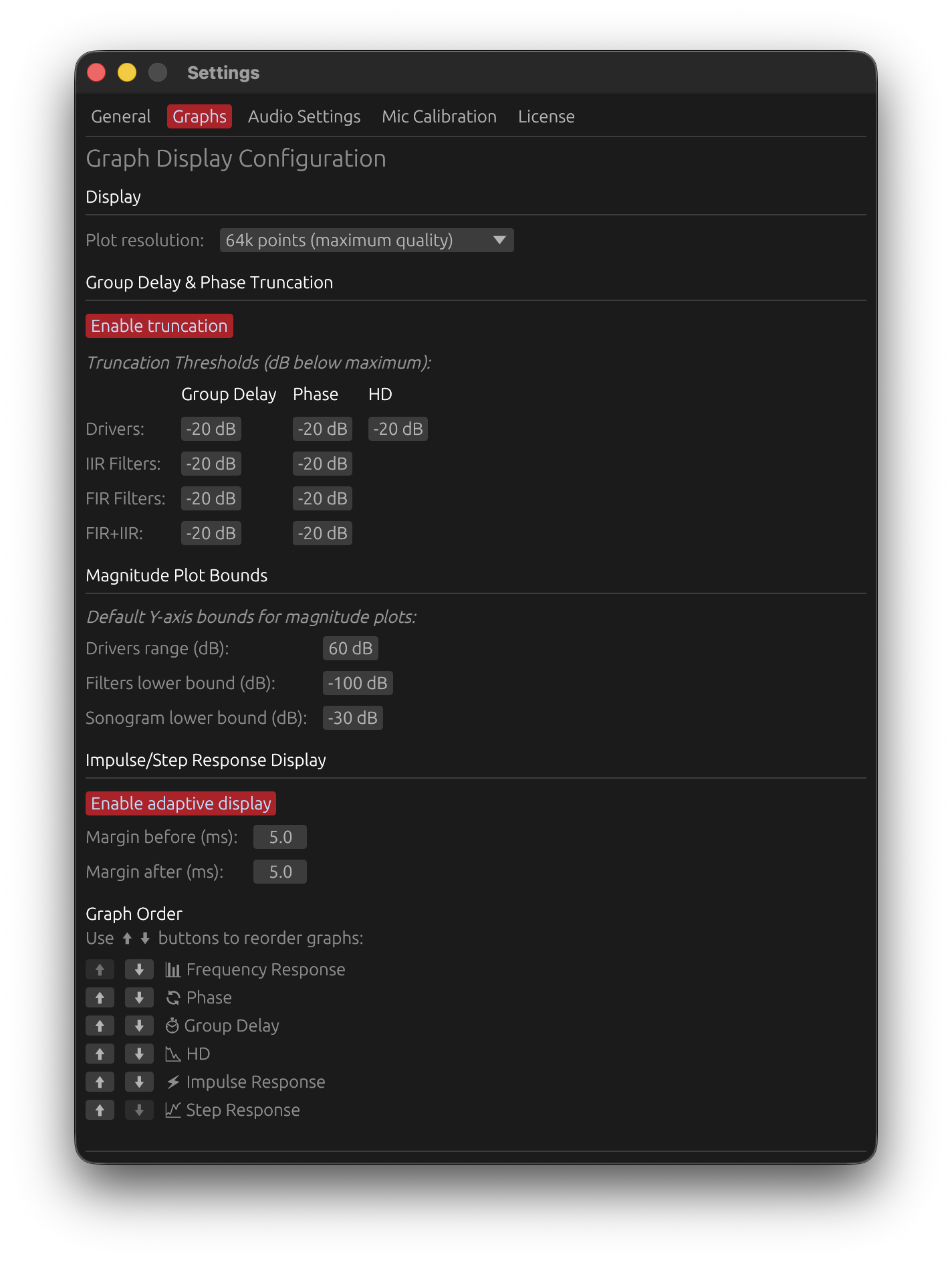
Graphs Settings
Configure display options and graph behavior.
Display
Plot Resolution
Options: 16k points, 32k points, 64k points
Default: 32k points (balanced)
FFT resolution for frequency response computation.
- 16k points (16384): Faster computation, lower frequency resolution
- 32k points (32768): Balanced performance and resolution
- 64k points (65536): Maximum frequency resolution, slower computation
Impact:
- Higher resolution provides finer low frequency detail in magnitude, phase, and group delay plots
- Affects computation time for filter responses and driver measurements
- Does not affect the actual filter quality, only the analysis resolution
Steep Crossover Smoothing
Options: Enabled, Disabled
Default: Enabled
Reduces smoothing near crossover frequencies to reveal steep filter slopes in magnitude plots.
How it works:
The strength of the smoothing reduction is proportional to the filter’s effective acoustic slope:
| Filter order / type | Slope | Smoothing reduction |
|---|---|---|
| 1st-order Butterworth | 6 dB/oct | None |
| LR2 / 2nd-order Butterworth | 12 dB/oct | None |
| 3rd-order Butterworth | 18 dB/oct | ~25 % |
| LR4 / 4th-order Butterworth | 24 dB/oct | ~50 % |
| 5th-order Butterworth | 30 dB/oct | ~75 % |
| LR6 / 6th-order Butterworth | 36 dB/oct | 100 % (down to 1/96 oct at Fc) |
| LR8 / higher order | ≥ 48 dB/oct | 100 % |
| Brickwall FIR | — | 100 % |
The transition is progressive: smoothing is gradually reduced within ±0.5 octave around the crossover frequency, reaching the minimum at Fc itself.
When enabled:
- Steep crossovers (LR6 / 36 dB/oct and above) receive full reduction — smoothing drops to 1/96 octave at Fc
- Common crossovers (LR4 / 24 dB/oct) receive an intermediate reduction of ~67 %
- Shallow crossovers (LR2 / 12 dB/oct and below) are left unchanged — the filter slope is gentle enough to be visible without smoothing reduction
- Brickwall FIR always use full reduction (safe default)
- Only affects magnitude display curves — does not modify phase, group delay, or filter generation
When disabled:
- Uniform smoothing is applied across the entire frequency range
- Provides consistency with external measurement tools that use constant smoothing
Note: External measurements with uniform smoothing will show gentler crossover slopes compared to LinFIR’s steep-crossover mode. This is expected — the adaptive reduction reveals the true filter response near crossovers.
Group Delay & Phase Truncation
Optionally truncate group delay and phase curves to the active frequency region using magnitude thresholds.
Enable Truncation
Default: Enabled
When checked: Group delay and phase curves are shown only where the corresponding magnitude exceeds a threshold below the maximum.
When unchecked: Full-range phase and group delay displayed regardless of magnitude.
Purpose:
- Avoid displaying phase/group delay in stop-band regions
- Focus on pass-band characteristics
- Reduce visual clutter from irrelevant frequency ranges
Truncation Thresholds (dB below maximum)
Independent thresholds for different contexts:
| Context | Group Delay | Phase | THD |
|---|---|---|---|
| Drivers | -20 dB | -20 dB | -20 dB |
| IIR Filters | -20 dB | -20 dB | — |
| FIR Filters | -20 dB | -20 dB | — |
| FIR+IIR | -20 dB | -20 dB | — |
How thresholds work:
- Values are expressed as dB below the maximum magnitude in the reference curve
- Example: -20 dB means “show phase/GD only where magnitude > (max - 20 dB)”
- Adjustable range: -120 dB to -20 dB
Context matching:
- The reference magnitude matches the context
- Example: FIR curves use FIR magnitude as reference
- Drivers use driver magnitude as reference
THD Truncation:
- Only available for Drivers context
- Shows Total Harmonic Distortion only in active magnitude regions
Magnitude Plot Bounds
Configure default Y-axis bounds for magnitude plots.
Drivers Range (dB)
Range: 20 to 200 dB
Default: 60 dB
Y-axis range for speaker magnitude plots.
- Calculation: From (max_response - range) to (max_response + 5 dB)
- Smaller values (20-40 dB): Zoomed view, emphasizes small variations
- Moderate values (60-80 dB): Good balance for most designs
- Larger values (100-200 dB): Wide view, shows full range
Filters Lower Bound (dB)
Range: -200 to 0 dB
Default: -100 dB
Lower bound of Y-axis for filter magnitude plots (IIR, FIR, FIR+IIR).
- Higher values (-40 dB): Focuses on pass-band details
- Lower values (-100 to -200 dB): Shows deep stop-band attenuation
Impulse/Step Response Display
Adaptive display automatically detects and shows only the relevant portion of impulse and step responses.
Enable Adaptive Display
Default: Enabled
When checked: Automatically detects signal boundaries based on amplitude threshold.
- Detection threshold: 1/1000th of peak amplitude
- Automatic margins: Adds configurable time before and after detected signal
When unchecked: Always shows the complete impulse response (full tap length).
Use case: Focuses view on active signal portion, especially useful for long impulse responses with significant zero-padding.
Margin Before (ms)
Range: 0 to 50 ms
Default: 5 ms
Time added before detected signal start.
Purpose: Ensures pre-ringing or early arrivals are visible in the plot.
Margin After (ms)
Range: 0 to 100 ms
Default: 10 ms
Time added after detected signal end.
Purpose: Captures decay tail and late reflections.
Focus on Summed Response
Default: Disabled
When enabled in multi-driver plots:
- All curves (individual drivers and sum) use the summed IR time boundaries
- Focuses on the main energy region of the system response
When disabled (default):
- Uses the union of all individual curve boundaries
- Shows the full extent of all driver responses
Use case: Quickly identify timing alignment issues across speakers by focusing on the system sum.
Response Overlays
Show Listening Window Curve
Default: Enabled
Requires: A valid LinFIR license
Displays the Listening Window curve in the frequency graph when in Drivers/Measurements mode and off-axis measurements are available. The curve appears in the graph legend as “LW”.
The Listening Window is the spatial average of responses within ±30° horizontal and ±10° vertical. See System Processing for details.
Note: This option is disabled when no valid license is present. The toggle is grayed out and the curve is not displayed.
Show Raw Response When Filter Windows Are Open
Default: Enabled
Requires: A valid LinFIR license
When enabled, a dashed overlay of the unfiltered (pre-filter) driver response is drawn on the frequency, phase, and group delay graphs whenever a filter window is open for that driver.
Which windows trigger the overlay:
- Per-driver: LP, HP, correction FIR, or IIR filter window
- Global: Global FIR correction or Global IIR filter window (shows the unfiltered sum/average)
What is shown:
- The response before any FIR or IIR filter is applied to that driver — the raw impulse response processed only through gain and windowing
- The overlay is colored to match the driver’s curve color, drawn as a thin dashed line
- For the global sum, the overlay is drawn in white (dark mode) or black (light mode)
Use case: Immediately see how much correction a filter is applying, without disabling filters. Useful for validating crossover slopes, EQ depth, and phase shaping against the unprocessed baseline.
Note: This option is disabled when no valid license is present. The toggle is grayed out and the overlay is not displayed.
Settings Summary Table
| Setting | Default | Purpose |
|---|---|---|
| Appearance | ||
| UI Color Scheme | Red | Interface accent colors |
| Theme | Follow System | Light/Dark mode |
| Filter Processing | ||
| Clipping Detection | Enabled | Safety warnings for filter output levels |
| Auto Causal Alignment | Enabled | Optimize IR positioning with causal filters |
| Show Manual FIR Delay Compensation | Disabled | ⚙️ Advanced: Show manual FIR delay fields |
| Default Values | ||
| Sample Rate | 48 kHz | Default for new projects |
| Speaker FIR Taps | 512 | Per-driver FIR filter length |
| Global FIR Taps | 512 | Global correction filter length |
| Curve Smoothing | 1/12 octave | Frequency response smoothing |
| Graph Display Mode | Drivers/Measurements | Initial display mode |
| Phase Display | Wrapped | Phase graph mode |
| Remove time of flight rotations | Disabled | Linear phase removal |
| Graphs | ||
| Plot Resolution | 64k points | Frequency point count |
| Steep Crossover Smoothing | Enabled | Reduce smoothing near steep crossover frequencies |
| GD/Phase Truncation | Enabled | Truncate by magnitude threshold |
| Truncation Thresholds | -20 dB | Threshold below max |
| Drivers Range | 60 dB | Y-axis range for drivers |
| Filters Lower Bound | -100 dB | Y-axis lower limit for filters |
| Adaptive IR Display | Enabled | Auto-detect IR boundaries |
| Margin Before | 5 ms | Pre-signal margin |
| Margin After | 10 ms | Post-signal margin |
| Focus on Summed Response | Disabled | Use sum boundaries for all curves |
| Response Overlays | ||
| Show Listening Window Curve | Enabled | Display Listening Window (“LW”) in Drivers mode (requires license) |
| Show Raw Response When Filter Windows Are Open | Enabled | Dashed pre-filter overlay on magnitude/phase/GD graphs (requires license) |
Performance Considerations
Real-Time Filter Processing Architecture
LinFIR differs fundamentally from traditional FIR filter design software in how it processes and displays results.
Real-time (“online”) filter generation:
- Filters are generated and applied to driver impulse responses in real time based on UI interactions
- The complete signal processing chain is computed immediately as you adjust parameters
- You see the true response of the entire filter chain instantly, including all windowing artifacts and actual behavior
Why this matters:
- Immediate feedback: No “generate” or “apply” button required - changes are visible instantly
- Transparency: Shows exactly what the filters can and cannot do, with all artifacts visible
- Accuracy: No approximation or preview mode - what you see is what you get
Contrast with traditional software:
- Most FIR design tools require you to validate parameters before showing the true response
- They often show theoretical or idealized responses that don’t reflect actual implementation artifacts
- LinFIR prioritizes showing real-world behavior over computational convenience
Filter Application Methods
FIR filters:
- Applied via fast convolution (multiplication in Fourier domain)
- Highly efficient for typical filter lengths
- Computational cost scales with filter length and number of measurements
IIR filters:
- Applied via recursive difference equations (time-domain processing)
- Extremely efficient regardless of filter complexity
- Minimal performance impact even with many cascaded sections
Performance Impact Factors
Filter length:
- Filters up to 4096 taps: Negligible performance impact on modern CPUs
- Filters 4096-8192 taps: May cause slight delays on slower systems
- Filters >8192 taps: Can noticeably slow down the application, especially during interactive adjustments
Off-axis measurements:
- Each off-axis measurement requires the full filter chain to be recomputed
- Projects with many off-axis angles and long filters may experience longer update times
- LinFIR prioritizes UI responsiveness using background processing (see below)
Background Processing for Responsiveness
To maintain smooth UI interaction even with complex projects, LinFIR uses processing prioritization:
Priority processing (synchronous, immediate):
- On-axis measurement (0°, 0°): Always computed first in the main thread
- Currently displayed angle: Computed immediately for instant visual feedback
- Filter parameters: Updated in real-time as you adjust controls
Background processing (asynchronous, non-blocking):
- Remaining off-axis measurements: Computed in a background thread after priority angles
- Directivity index: Calculated asynchronously when all measurements are ready
- System sum calculations: Processed in parallel when multiple drivers are active
User experience:
- Main graph updates are always immediate - you see changes to the selected angle instantly
- UI remains fully responsive even during heavy background computations
- You can continue adjusting parameters while background calculations complete
Optimization Recommendations
For slower systems or very long filters (>8192 taps):
-
Reduce plot resolution: Settings → Graphs → Plot Resolution
- Default: 64k points (maximum quality)
- Recommended for performance: 16k or 32k points
- Performance improvement with minimal visual quality loss
-
Disable clipping detection: Settings → General → Filter Processing
- Eliminates test signal processing on every update
- Only disable if you’re confident in your gain staging
-
Limit off-axis measurements:
- Use reasonable angle increments (10 or 15°)
Performance is always optimal for:
- Projects with standard filter lengths (≤4096 taps)
- IIR-only filtering (always fast regardless of complexity)
- Single on-axis measurements
- Modern multi-core processors (2020 or newer)
Best Practices
Performance Optimization
- Slower systems: Reduce plot resolution to 16k or 32k points
- Complex projects: Consider disabling clipping detection if filters are well-understood
Filter Design
- Auto Causal Alignment: Keep enabled unless you need precise manual control over IR positioning
- Show Manual FIR Delay Compensation: Keep disabled unless you are experienced in signal processing and need manual FIR alignment control
- Clipping Detection: Keep enabled during design, test actual content before deploying
Graph Display
- Truncation: Enable for cleaner phase/GD plots focused on active frequency regions
- Focus on Summed Response: Enable when analyzing multi-driver timing alignment
Measurement Setup
- Sweep Duration: Use 5-7 seconds for full-range, 2-3 seconds for limited bandwidth
- Sweep Level: Adjust based on amplifier sensitivity (-12 to -6 dBFS typical)
Audio Configuration
Before performing measurements or analyzing audio, LinFIR needs to be configured with the correct audio devices and parameters. This section covers the audio settings available in the application.
Accessing Audio Settings
Audio settings are accessed via:
- Menu: View → Settings → Audio Settings
- Keyboard: Cmd+, (macOS) or Ctrl+, (Windows), then select Audio Settings tab
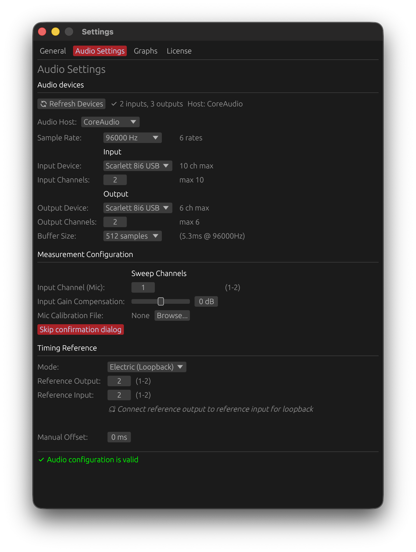

Device Selection
Input Device
The input device captures audio from microphones or measurement equipment:
- Click the dropdown to see available input devices
- Select your measurement microphone or audio interface input
- Verify the device shows the correct channel count
- Ensure the device isn’t in use by another application
Output Device
The output device plays back sweep signals or test tones:
- Select the audio interface connected to your loudspeaker system
- Verify the device supports the desired sample rate
- Check that the device has sufficient channels for your application
Refreshing Devices
If your audio device doesn’t appear:
- Click “Refresh Devices” to rescan available hardware
- Ensure the device drivers are properly installed
- Check that the device is powered on and connected
- Try restarting the application if the device remains unavailable
Sample Rate Configuration
Choose a sample rate matching your needs:
- 44.1 kHz: CD quality, most common for consumer audio
- 48 kHz: Professional audio standard, video production
- 88.2/96 kHz: High-resolution audio, improved time-domain precision
- 176.4/192 kHz: Ultra-high resolution (use only when necessary for THD analysis)
⚠️ Note: The sample rate must be supported by both your input and output devices. If a rate is unavailable, try a different value.
Sample Format Detection
LinFIR automatically detects and selects the best compatible audio sample format between your input and output devices:
- 16-bit integer (I16): Standard for most consumer audio devices
- 24-bit integer (I24): Professional audio interfaces (e.g., Dante Virtual Soundcard, RME, MOTU)
- 32-bit float (F32): High-end interfaces, ASIO and Core Audio devices
- 32-bit integer (I32): Some professional hardware
The format is automatically negotiated during measurement setup - no manual configuration required. If LinFIR cannot find a compatible format, try:
- Using ASIO drivers (Windows) for better professional interface support
- Updating your audio interface drivers
- Checking device sample rate compatibility
Buffer Size
Buffer latency is compensated internally and has no effect on measurement accuracy. The only criterion for choosing a buffer size is avoiding underruns (audio dropouts caused by the buffer emptying before it can be refilled).
- Smaller buffers (128-256 samples): More demanding on the CPU — increase the risk of dropouts on slower systems
- Recommended (512-1024 samples): Reliable on most systems
- Larger buffers (2048+ samples): Maximum stability, useful if dropouts persist
If you experience audio dropouts during measurements, increase the buffer size. Otherwise, any value works.
Input Gain Compensation
Software-based gain adjustment applied to the input signal:
- Range: -32 dB to +32 dB
- Purpose: Compensate for fixed or unavailable hardware gain controls
- Use case: Particularly useful for USB microphones like UMIK-1 on Mac OS
Why Use Input Gain Compensation?
Some measurement microphones have fixed gain or no hardware gain control, particularly on certain platforms:
- Mac OS USB microphones: Mac OS enforces very low fixed gain for USB microphones
- UMIK-1 example: No hardware control available in Mac OS system settings
- Solution: Use positive gain compensation (+18 to +24 dB) to achieve optimal recording levels
Important Notes
- Input gain compensation does not improve signal-to-noise ratio
- It’s a convenience feature for level matching, not a replacement for proper gain staging
- Optimal SNR still requires appropriate acoustic levels and microphone positioning
- Use hardware gain controls when available for best results
Default Sweep Parameters
Configure default settings for the built-in sweep measurement system. These apply to new measurement captures and can be accessed in the Audio Settings tab under Measurement Configuration.
Sweep Duration
Range: 1.0 to 10 seconds
Default: 5 seconds
Default length of exponential sine sweep (ESS) for impulse response measurements.
- Shorter (1.0-2s): Faster measurements, lower frequency resolution
- Longer (5-10s): Better low-frequency resolution, improved signal-to-noise ratio, better harmonic distortion measurement
Benefits of longer sweeps:
- Improved signal-to-noise ratio for harmonic distortion analysis
- Better frequency resolution at low frequencies
- More reliable detection and separation of weak harmonics
⚠️ Important: Longer sweeps deliver more energy to the driver at low frequencies (exponential sweeps spend more time in the bass region). For drivers with limited excursion capability, this may require raising the start frequency or reducing the sweep level to avoid over-excursion.
Recommendation: 5-7 seconds for full-range measurements, 2-3 seconds for quick driver checks.
Sweep Level
Range: -40 to 0 dBFS
Default: -6 dBFS
Default output level for sweep signals.
Adjust this to match your amplifier’s input sensitivity and desired acoustic level. Lower values provide headroom for systems with high gain.
Start Frequency
Range: 1 to 5000 Hz
Default: 1 Hz
Default cutoff frequency for the 4th-order Butterworth high-pass filter applied to the sweep signal for driver protection.
Filter Characteristics:
- Attenuation at Start Frequency: -3 dB (Butterworth characteristic)
- Roll-off below cutoff: -24 dB/octave (deterministic, 4th order)
Frequency Guidelines:
- 1 Hz: Lowest configurable frequency, captures near-DC response
- 20 Hz: Typical for full-range loudspeaker measurements
- 60-70 Hz: Example for 80 Hz passband (accounts for -3 dB at cutoff)
- >1000 Hz: Tweeter protection (above resonance frequency)
⚠️ Critical: Position Start Frequency slightly below your desired passband start to compensate for the -3 dB attenuation at cutoff, but always above driver safety limits. Setting too low can cause mechanical or thermal damage.
See Start Frequency: Driver Protection for detailed guidance on driver-specific settings.
Note on high frequency: The high frequency is automatically calculated to optimize harmonic distortion measurement quality (1/48 octave before Nyquist), typically ~23.5 kHz at 48 kHz sample rate, ~47 kHz at 96 kHz.
Using Default Values
These default values are applied when:
- Opening a new measurement window for the first time
- Clicking the Reset Start Freq button in the measurement window
- Creating a new driver without saved sweep parameters
Changing these defaults affects only future measurements - existing measurements retain their configured parameters.
Platform-Specific Considerations
Mac OS
- Timing stability: Excellent (< 0.01ms typical jitter)
- Timing reference: Optional when the same device is used as input and output but recommended for best accuracy
- Multi-interface: Highly reliable even with different input/output devices
- USB microphones: May require input gain compensation due to OS-enforced low gain with usb devices
Windows
- Timing stability: Variable (1-150ms jitter due to scheduler instability)
- Timing reference: Strongly Recommended (Electric or Acoustic mode) for absolute timing accuracy
- Timing inconsistency: IR arrival time may vary without timing reference
- ASIO drivers: Provide improved stability compared to WASAPI
- Measurement averaging: Works with or without timing reference (continuous capture method)
A timing reference on Windows improves absolute timing consistency when comparing measurements across drivers.
Configuration Checklist
Before starting measurements, verify:
- Input device selected and recognized
- Output device selected and functional
- Sample rate matches project settings
- Buffer size set to 256 or 512 samples
- Input gain compensation configured (if needed)
- Microphone calibration loaded (if available)
- Timing reference configured (see Reference Timing below)
- Devices not in use by other applications
Reference Timing for Sweep Measurements
Accurate timing is critical for consistent impulse response measurements, especially when capturing multiple measurements for averaging or multi-position analysis. LinFIR provides three timing reference modes to accommodate different hardware configurations and platform requirements.
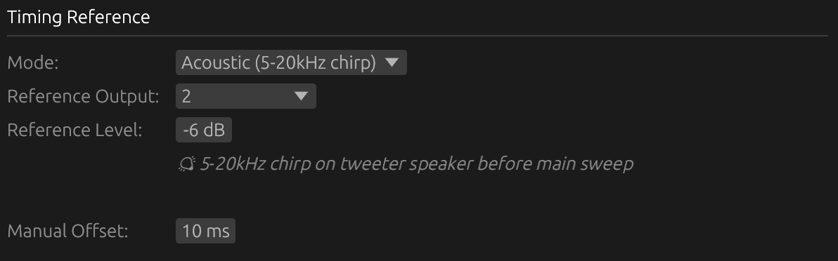
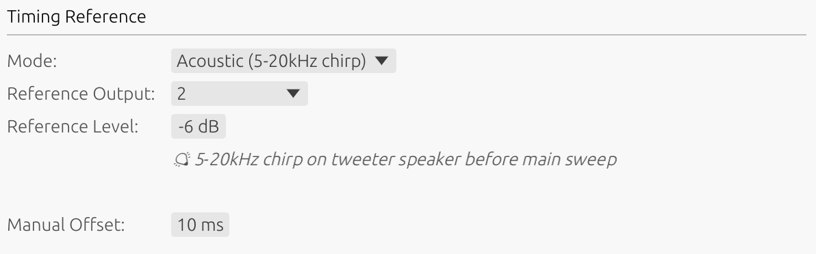
Why Timing Reference Matters
Audio playback and recording systems introduce latency from:
- Digital-to-analog conversion (output)
- Analog-to-digital conversion (input)
- Buffer processing delays
- Operating system scheduler variability
Without a stable timing reference, each measurement may have slightly different latency, making:
- Driver alignment unreliable
- Directivity analysis inaccurate (time-of-flight variations)
Timing Reference Modes
None
No timing reference - relies solely on system scheduler timestamps.
How it works:
- Uses operating system audio clock
- Timestamps based on buffer callback timing
- No additional hardware or connections required
When to use:
- Mac OS systems (low scheduler jitter, typically < 0.01 ms)
- Single-shot measurements without averaging
- Simple setups where high precision isn’t critical
Limitations:
- Windows: Not recommended due to significant scheduler jitter (1-150 ms)
- IR arrival time may vary between captures
Mac OS: Reliable and accurate for most applications when using the same device as input and output. Windows: Avoid for professional work - use Electric or Acoustic mode instead.
Electric (Loopback)
Uses a physical cable connection between output and input to provide a stable timing reference.
How it works:
- Connect line output to line input with a cable
- Loopback signal captures exact OS and electrical latency
- Combined electrical and conversion latency measured
- Provides sample-accurate timing reference
Setup:
- Connect output channel to spare input channel with audio cable
- Select “Electric” timing reference mode in Audio Settings
- Ensure loopback channel is not the measurement input channel
- Run sweep - loopback captures timing automatically
Advantages:
- Most accurate timing reference
- Platform-independent reliability
- Compensates for interface-specific latency
- Eliminates scheduler jitter completely
When to use:
- Windows systems (strongly recommended)
- Designing crossovers
- Professional applications requiring highest accuracy
- Different input/output devices (aggregate devices)
Limitations:
- Requires spare input channel for loopback
- Requires physical cable connection
- May not be available on simple USB audio interfaces
Acoustic
Uses another driver (reference driver) as a timing microphone.
How it works:
- Reference driver captures sweep output acoustically
- Provides stable timing reference based on acoustic arrival
- Measures relative timing between reference and measured driver
- Does not capture true absolute acoustic + electrical travel time
Setup:
- Select a reference driver (must reproduce high frequencies > 5 kHz)
- Position reference driver microphone to capture sweep clearly
- Select “Acoustic” timing reference mode in Audio Settings
- Reference driver captures timing on each sweep
Advantages:
- No loopback cable required
- Works when electrical loopback unavailable
- Good alternative for Windows users without spare input channels
- Suitable for multi-driver directivity measurements
When to use:
- Loopback hardware not available
- Windows systems (recommended alternative to None)
Limitations:
- Only measures relative timing (not absolute acoustic delay)
- Reference driver must reproduce high frequencies cleanly
- Acoustic path must be clear and consistent
- Less accurate than Electric mode
Important: Reference driver should be full-range or at least capable of reproducing 5-10 kHz cleanly for reliable timing detection.
Manual Offset (Preferences)
Adjustable time offset to shift the impulse response position.
- Range: ±4000 ms
- Applies to: All timing reference modes (None, Electric, Acoustic)
- Purpose: Shift the IR forward or backward in time
Use in all modes (convenient)
The offset can be used in any timing mode to position the IR at a convenient location in the window — for example, to center it or add pre-delay before a gate. This is optional and has no impact on accuracy.
⚠️ Caution: A positive offset shifts the IR earlier in the window. If the offset is too large (positive), the impulse peak may move before t=0 and be clipped. Keep the offset small enough to leave sufficient pre-delay in front of the impulse.
Use in Acoustic mode (required in certain cases)
In Acoustic mode, the timing reference is based on the acoustic arrival at the reference driver. If the reference driver is at a similar or shorter distance from the microphone than the measured driver, the IR of the measured driver will appear at time zero or even before it — making it impossible to capture the full impulse response.
In this case, a positive offset must be applied to shift the IR forward and restore the expected relative delay.
Example — reference closer than measured driver:
- Reference driver is 150 cm from the microphone
- Measured driver is 200 cm from the microphone
- Acoustic delay difference ≈ 1.5 ms (50 cm / 343 m/s)
- Apply a positive offset just above ~1.5 ms — large enough to place the impulse response after t=0 with a safety margin
- Use the same offset, mic distance, and reference driver for all measurements in the project — since the offset is constant, the relative acoustic delay between drivers is preserved, enabling accurate temporal alignment when designing crossovers
Fine-tuning:
- Run test measurement
- Check impulse response time alignment
- Adjust offset in small increments
- Re-measure to verify alignment
Platform Requirements
Windows
- Averaging: Works with or without timing reference (continuous capture eliminates jitter issues)
- Scheduler jitter: Significant (1-150 ms variable latency) for initial timing only
- Recommendation: Timing reference still recommended for absolute timing accuracy across sessions
- Single measurements: Work with “None” mode but may have timing variation
Without timing reference on Windows:
- Each measurement has unpredictable latency
- Directivity analysis compromised
- Time and phase alignment between drivers will lead to wrong results
Mac OS
- Scheduler jitter: Minimal (< 0.01 ms typical)
- Recommendation: Timing reference optional but still beneficial for best accuracy
- Multi-interface: More stable than Windows even without reference
Choosing the Right Mode
| Situation | Recommended Mode |
|---|---|
| Windows + single shots | Acoustic or Electric (None acceptable) |
| Mac OS + single shots | None acceptable, Electric for best accuracy |
| Different input/output devices | Electric strongly recommended |
| Directivity measurements | Electric or Acoustic |
| Crossover design | Electric or Acoustic |
| No spare input channel | Acoustic (Windows) or None (Mac OS) |
Configuration Workflow
-
Assess requirements:
- Single measurement or averaging?
- Mac OS or Windows?
- Spare input channel available?
-
Select mode:
- Windows averaging → Electric or Acoustic
- Mac OS → None acceptable, Electric for best results
- No loopback → Acoustic (if reference driver available)
-
Setup hardware (if Electric):
- Connect output to spare input channel
- Verify loopback signal path
-
Setup reference driver (if Acoustic):
- Select driver with good high-frequency response
- Position reference microphone to capture sweep clearly
-
Configure in Audio Settings:
- Select timing reference mode
- Adjust timing offset if needed (Acoustic mode)
-
Test:
- Run test measurement
- Verify timing consistency
- Adjust offset if required
Timing Reference Troubleshooting
Inconsistent Measurements
Symptom: Each measurement has different arrival time
Cause: No timing reference active
Solution: Enable Electric or Acoustic mode
Reference Signal Not Detected
Symptom: Error message about missing reference
Cause: Loopback not connected or reference driver not capturing sweep
Solution:
- Electric: Verify cable connection and input channel selection
- Acoustic: Ensure reference driver can reproduce sweep frequencies
Timing Offset Not Working
Symptom: Impulse still misaligned after offset adjustment
Cause: Incorrect offset direction or magnitude
Solution:
- Try opposite sign (positive ↔ negative)
- Increase offset magnitude
- Verify reference driver is capturing sweep correctly
Best Practices
- Windows users: Always use Electric or Acoustic mode for professional work
- Loopback preferred: Most accurate, eliminates all timing variables
- Acoustic alternative: Good fallback when loopback unavailable
- Test before session: Verify timing consistency with test measurements
- Document settings: Record timing mode and offset in project notes
- Consistent hardware: Use same interface for all measurements in a session
Troubleshooting
Device Not Listed
- Click “Refresh Devices” to rescan
- Ensure device drivers are installed
- Check that device isn’t in use by another application
- Try different sample rates or buffer sizes
- Restart LinFIR
Configuration Invalid
- Selected devices may have been disconnected
- Sample rate may not be supported by device
- Channel count may exceed device capabilities
- Try selecting default devices and refreshing
Audio Dropouts
- Increase buffer size
- Close other applications using audio
- Check for system resource constraints
- Update audio interface drivers
No Sound During Sweep
- Verify output device is selected and powered on
- Check system audio settings
- Ensure exclusive mode isn’t blocking access (Windows)
- Try different buffer sizes
- Verify output channel selection in IR Management window
Microphone Calibration
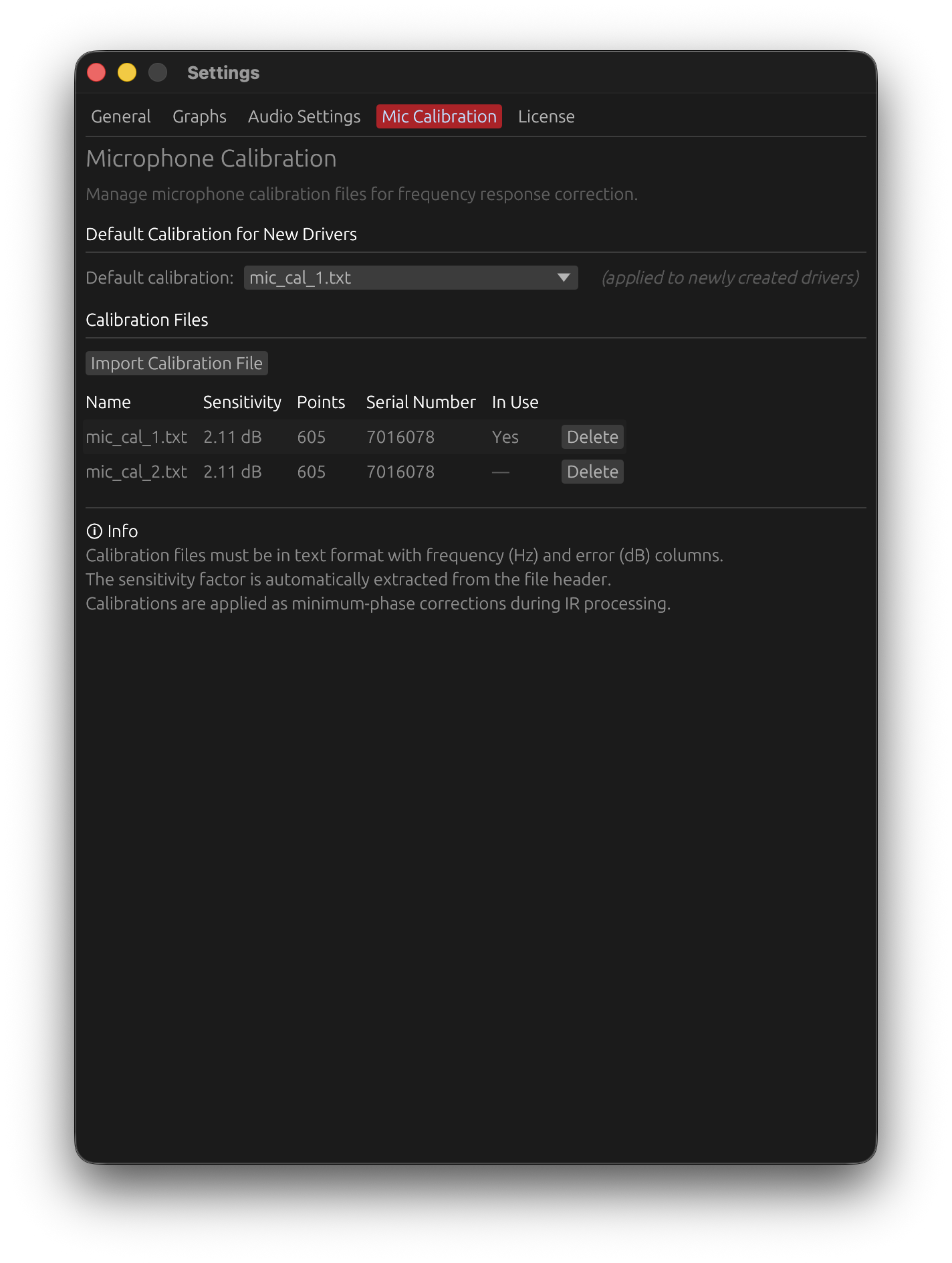
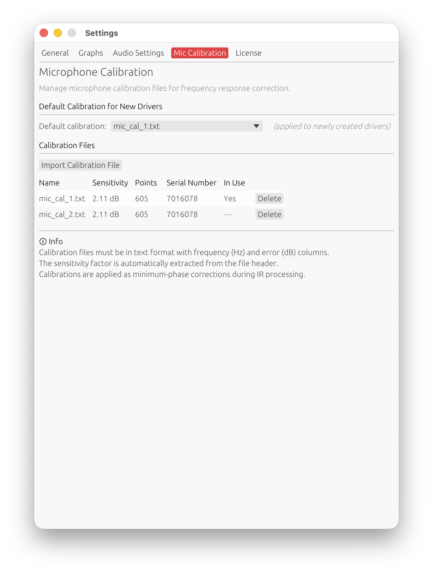
Manage calibration files for measurement microphones and define default calibrations for new drivers.
Overview
Microphone calibration compensates for the frequency response and sensitivity of your measurement microphone. LinFIR supports:
- Multiple calibration files stored in application settings
- Per-driver calibration selection in the IR Management window (see IR Management)
- Default calibration for newly created drivers
- Automatic application to new projects when a default is set
- Minimum-phase correction computed in real-time from calibration data
Calibration scope:
- Calibration data is embedded in project files (
.lnf) for portability - Calibrations from projects are also stored in application settings for reuse
- Each driver can use a different calibration file or none at all
Calibration File List
The main section displays all imported calibration files in a scrollable grid:
| Column | Content |
|---|---|
| Name | Filename without extension |
| Sensitivity | Microphone sensitivity factor in dB |
| Frequency Points | Number of frequency/magnitude pairs in the file |
| Serial Number | Microphone serial number (if present in file), empty otherwise |
| In Use | Yes if used in current project (hover to see driver names), empty otherwise |
| Actions | Delete button (🗑️) to remove the calibration |
Automatic driver updates:
- When you delete a calibration file that’s currently assigned to one or more drivers, those drivers are automatically reset to “None”
- A warning toast will notify you which drivers were affected
- This prevents broken references and ensures project stability
Default Calibration
Select a calibration file to automatically apply to newly created drivers.
Dropdown selector:
- Shows “None” when no default is set
- Lists all imported calibration files by name
- Changes apply immediately to new drivers and projects
When the default is applied:
- Manual driver creation: When you add a new driver via the Drivers toolbar
- New Loudspeaker Design project: All initial drivers receive the default calibration
- New Room Calibration project: The initial measurement receives the default calibration
Note: Changing the default does not affect existing drivers in the current project or previously saved projects. Only new drivers created after the change receive the new default.
Import Calibration File
Click “Import Calibration File” to load a microphone calibration file.
Supported file format:
- Plain text files with two or three columns: Frequency (Hz), Magnitude (dB), and optionally Phase (degrees)
- Whitespace or comma-separated
- Lines starting with non-numeric characters are treated as comments/headers
- Optional header line with sensitivity factor and serial number
Note on phase column: If a third column (phase) is present, it is intentionally ignored. Phase data exported by calibration software is typically smoothed, wrapped, or otherwise processed in ways that make it unsuitable for direct use in transfer function reconstruction. Since measurement microphones exhibit predominantly minimum-phase behavior, reconstructing the phase from the magnitude alone (via Hilbert transform) is both accurate and more robust than relying on the exported phase values.
Example file format:
# Sens Factor = -2.5dB, SERNO: 41486651
# Frequency (Hz)  Magnitude (dB)
20.0              -0.5
50.0              -0.3
100.0             -0.1
200.0              0.0
500.0              0.1
1000.0             0.0
2000.0            -0.2
5000.0            -0.5
10000.0           -1.0
20000.0           -2.0
Sensitivity factor and serial number:
- Sensitivity factor (in dB) is automatically extracted from the file header if present (line containing “Sens Factor”)
- Serial number is automatically extracted if present (SERNO: field in header)
- If no sensitivity factor is found in the file, it defaults to 0 dB
- Serial number is used to differentiate calibrations with identical filenames when sharing projects
Storage:
Calibration data (frequency response, sensitivity, and serial number) is embedded in project files (.lnf) to ensure portability:
- Projects can be shared without requiring recipients to have the calibration files
- When loading a project, calibrations are automatically added to application settings if not already present
- If a calibration with the same name exists:
- With serial number: differentiated using serial number (e.g.,
filename (SN:7016078)) - Without serial number: differentiated using numeric suffix (e.g.,
filename (1),filename (2))
- With serial number: differentiated using serial number (e.g.,
- You can also manually import calibrations to your settings library for reuse across projects
How Calibration is Applied
Minimum-phase correction: LinFIR converts the imported frequency response correction into a minimum-phase FIR filter applied during IR processing.
Processing steps:
- Frequency filtering: Bins below 5 Hz are removed to prevent phase distortion at very low frequencies
- Interpolation: Calibration data is interpolated to match your IR’s sample rate and FFT size
- Minimum-phase conversion: Magnitude correction is converted to minimum-phase using Hilbert transform
- Sensitivity compensation: The sensitivity factor (dB) is applied as a gain adjustment
- IR application: The resulting correction filter is convolved with the driver’s impulse response
Phase behavior: LinFIR does not use phase data from calibration files, even when present. Instead, the correction filter’s phase is reconstructed from the magnitude response via the Hilbert transform (cepstral minimum-phase lifting). This is intentional:
- Phase columns in calibration files are typically smoothed, wrapped, or quantized by the calibration software, and directly applying such data would introduce artifacts.
- Measurement microphones exhibit predominantly minimum-phase behavior in their frequency response deviations, meaning the phase is largely determined by the magnitude — making reconstruction accurate without measured phase.
The resulting correction therefore affects both magnitude and phase of the measurement, with the phase derived from minimum-phase theory rather than read from the file.
Per-Driver Calibration Selection
Each driver can use a different calibration file (or none). To assign a calibration to a specific driver, use the microphone calibration dropdown in the IR Management window.
See: IR Management → Microphone Calibration
Best Practices
File organization:
- Use descriptive filenames that include microphone model and serial number
- Example:
UMIK-1_SN123456.txtorEarthworks_M30_SN789.txt
Calibration maintenance:
- Import calibration files for all your measurement microphones
- Set your most frequently used microphone as the default
Project workflow:
- Assign calibrations in the IR Management window after importing measurements
- Use “None” for measurements taken with already-flat reference microphones
- Different drivers in the same project can use different calibrations (useful when combining measurements from multiple sessions)
Frequency range:
- Ensure calibration files cover the full measurement bandwidth
- LinFIR interpolates between provided points, but extrapolation beyond the calibration range may produce inaccurate results
- Most measurement microphones provide calibration data from 20 Hz to 20 kHz
Sensitivity factor:
- Use the value from your microphone’s calibration certificate
- This is typically a negative dB value (e.g., -0.5 dB, -2.4 dB)
- If unsure, use 0 dB and rely solely on the frequency response correction
Rotation Table
The Rotation Table settings panel lets you connect and control a motorized turntable for automated polar measurements. Once connected, the table integrates with the IR Management window to drive the auto-scan feature, which rotates the speaker and captures impulse responses at each angle without any manual intervention.
Requires a valid LinFIR license. All rotation table features — connection, manual jog controls, position dial, and auto-scan — are available to license holders only. Without a valid license the Settings → Rotation Table tab is displayed grayed out.
Supported Hardware
LinFIR supports two families of rotation table controllers:
| Controller | Interface | Detection | Example hardware |
|---|---|---|---|
| Pololu Tic (T500, T834, T825, T249, 36v4) | USB (native) | Automatic via USB VID/PID | Any stepper with a Tic controller |
| GRBL (Arduino) | USB-serial | Serial port enumeration | Audiomatica Medusa, DIY Arduino build |
Pololu Tic controllers are identified automatically by their USB vendor ID. GRBL boards appear as serial ports; LinFIR probes them with a status query to confirm the firmware.
Accessing the Settings
Open Edit → Settings (or Cmd+, / Ctrl+,) and select the Rotation Table tab.
Connecting a Table
1. Port and Baud Rate
LinFIR scans available ports each time the settings panel is drawn. Use the port combobox to select the device; the detected controller type is shown next to each entry (e.g. COM3 — GRBL or /dev/cu.usbmodem… — Pololu Tic).
For GRBL boards, choose the baud rate that matches your firmware (typically 115200). Pololu Tic controllers connected over USB do not use a baud rate.
A small label below the combobox confirms the auto-detected type:
Detected: GRBL
or
Detected: Pololu Tic
2. Connect / Disconnect
Click Connect to open the connection. LinFIR probes the controller and updates the detected type if needed. A status indicator appears to the right of the Disconnect button:
| Dot colour | Meaning |
|---|---|
| 🟢 Green | Connected — table idle |
| 🟡 Yellow | Table is moving |
Click Disconnect to cleanly close the serial/USB connection.
Position Dial
After connecting, a dial shows the current table angle:
- Red needle points to the current position (−180° to +180°)
- Cardinal labels: 0°, 90°, 180°, −90°
- ↻ button — sends a position query and refreshes the display immediately
The angle is updated automatically whenever the table moves or reports its position.
Manual Controls
GRBL Controllers
| Control | Description |
|---|---|
| Go to angle field + Go | Sends G1X<angle>F360 — moves to the specified angle at 360 deg/min |
| Set 0° at current position | Sends G92X0 — redefines the current position as the zero reference |
The Go button is disabled while the table is moving.
Pololu Tic Controllers
| Control | Description |
|---|---|
| Range — min / max steps | Defines the microstep positions that correspond to −180° and +180°. Drag-adjust or type a value. |
| Steps/° info label | Computed from the range: (max − min) / 360. Shown in grey below the range fields. |
| Go to angle field + Go | Converts the angle to microsteps using the range and sends SET_TARGET_POSITION |
| Set 0° at current position | Sends HALT_AND_SET_POSITION 0 — resets the current position to 0 steps / 0° |
Tic range calibration: Set the range so that the min and max step values span a full 360° rotation. For example, if your Tic is configured for 200 steps/rev × 16 microsteps = 3200 steps/rev, use −1600 to +1600 for ±180°.
Workflow: Manual Polar Measurement
If you prefer to position the table by hand and measure angle-by-angle without auto-scan:
- Connect the table in Settings → Rotation Table.
- Open the IR Management window for a driver.
- Use Go to angle to move the table to the desired off-axis angle.
- Set the Measurement angle field in the IR window to match.
- Click 🎤 Measure to capture.
- Repeat for each angle.
For a fully automated workflow, see Auto-Scan with a Rotation Table in the Sweep Measurements documentation.
Tips and Best Practices
- Set zero before scanning — use “Set 0° at current position” with the speaker pointing directly at the microphone, so 0° = on-axis.
- Always capture on-axis (0°) first — LinFIR requires a 0° reference before allowing off-axis measurements. If 0° is in the scan range it will be measured first automatically.
- Use a timing reference — for accurate phase relationships between angles, configure an Electric (loopback) or Acoustic timing reference in Audio Settings. This is critical for Directivity Analysis.
- Keep the mic at constant distance and height for all angles.
- 10° step or finer gives good sonogram and DI resolution. 5° is ideal.
- For the Pololu Tic, calibrate the step range carefully: a wrong range shifts all angle positions.
Troubleshooting
| Symptom | Likely cause | Fix |
|---|---|---|
| No port detected | Device not connected or driver missing | Plug in, install drivers, click away and back to refresh |
| “Auto-scan: rotation table timed out” | Table didn’t reach target in 30 s | Check wiring, reduce load, increase motor current |
| Table moves but angle stays 0° | Tic range is 0 (min = max) | Set correct min/max steps in Settings → Rotation Table |
| GRBL: table doesn’t respond to “Go” | Wrong baud rate | Try 9600 or 115200; match your firmware setting |
| Auto-scan skips some angles | Those angles already have a measurement | Delete existing measurements at those angles first |
Related Documentation
- Directivity Analysis — using polar measurements for DI and sonograms
- Sweep Measurements — sweep parameters and capture workflow
- Audio Setup — timing reference configuration
License
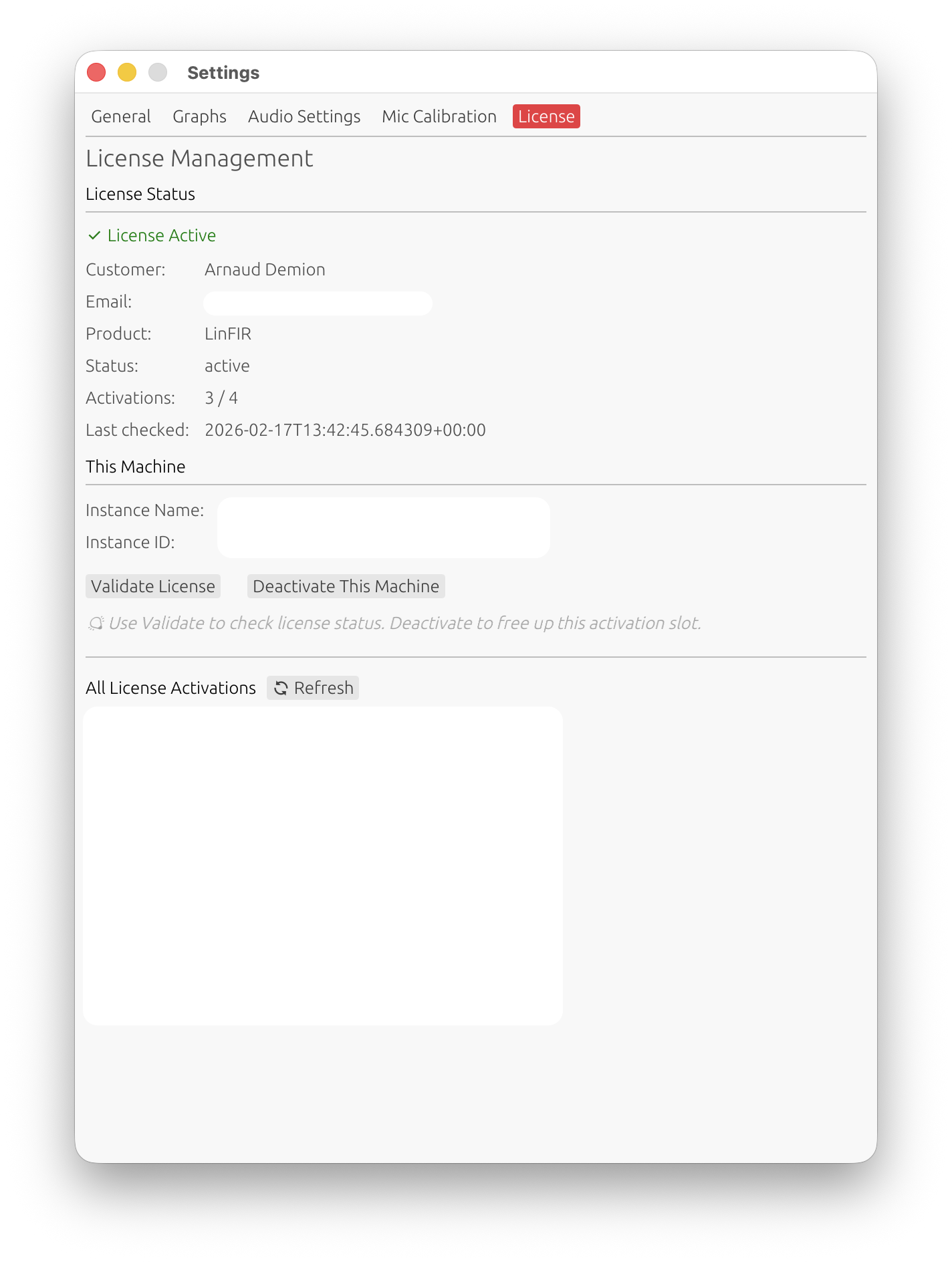
The License tab allows you to activate and manage your LinFIR license.
License Features
A valid LinFIR license unlocks advanced analysis features:
- Off-axis measurements: Import and analyze measurements at angles other than 0° (horizontal and vertical)
- Directivity Index (DI): Calculate and visualize directivity patterns across frequency
- Directivity Analysis: Access the Directivity Analysis window (sonogram and overlay plot) for detailed directivity visualization
- Spectrogram: Access the Spectrogram window (shortcut W) for time-frequency visualisation of the impulse response
- Multi-angle visualization: View multiple measurement angles simultaneously in graphs
- Pre-filter response overlays: When a FIR or IIR filter configuration window is open, a dashed overlay of the unfiltered speaker response (magnitude, phase, and group delay) is displayed on the corresponding graph, making it easy to compare the raw and filtered curves without toggling filters on and off
- Auto EQ — Auto-generate: The Auto-generate toggle in the IIR Auto EQ tab (per-driver and global) automatically re-runs the EQ optimization whenever any parameter in the Auto EQ tab changes, removing the need to manually trigger a recalculation
- Harmonic distortion details: View individual harmonic levels (THD breakdown by harmonic)
- Hypex FusionAmp mode: Create projects for Hypex FA series amplifiers with hardware-locked parameters and HFD export
Without a license, LinFIR operates with full functionality for on-axis measurements only (0°, 0°). The following features are unavailable without a license: off-axis analysis, directivity tools (DI, sonogram and overlay plot), spectrogram, pre-filter response overlays, Auto EQ auto-generate, harmonic distortion breakdown by harmonic, and Hypex FusionAmp project creation.
Activating Your License
If you don’t have an active license, the License tab will display an activation form.
Activation Process
-
Enter your license key
- Format:
xxxxxxxx-xxxx-xxxx-xxxx-xxxxxxxxxxxx - Provided in your purchase confirmation email
- Format:
-
Enter your email address
- Must match the email used for purchase
- Used for license validation
-
Click “Activate License”
- Creates a new activation tied to this specific machine
- Each activation is identified by a unique instance name and ID
Important:
- Each license allows one activation at a time
- Each activation is machine-specific
- You must deactivate one machine before activating another
- You can manage activations from the License tab
License Status
When a license is active, the License tab displays:
Current License Information
- Customer name: License holder’s name
- Email: Email address associated with the license
- Product: LinFIR license type
- Status: Current license status (active, expired, etc.)
- Activations: Number of active machines (e.g., “1 / 1”)
- Last checked: Date and time of last validation
This Machine
- Instance Name: Automatically generated name for this activation
- Instance ID: Unique identifier for this machine’s activation
Managing License Activations
Validate License
Click “Validate License” to check the current status of your license with the licensing server.
Use cases:
- Verify license is still active
- Update activation count
- Check for license changes
Deactivate This Machine
Click “Deactivate This Machine” to free up this activation slot.
When to use:
- Switching to a different computer
- Freeing up an activation for another machine
- System reinstall or hardware change
Effect:
- Removes this machine’s activation
- Frees one activation slot
- License features will no longer be available on this machine
- You can reactivate on this or another machine later
Managing Other Activations
The “All License Activations” section displays all machines where the license is currently active.
For each activation:
- Name: Instance name
- Instance ID: Unique identifier
- Created: Activation date
Actions:
- This Machine: Marked with ✓ (cannot be deactivated from this view)
- Other machines: Click “Deactivate” to remove that activation remotely
Use case: If you activated LinFIR on a machine you no longer have access to, you can deactivate it from here to free up that slot.
Troubleshooting
Unable to reach the license server
Symptoms: Activation fails with a message about a network proxy, firewall, or “temporarily unavailable”.
Causes: The license server is protected by Cloudflare. A corporate firewall, VPN, proxy, or content filter may intercept the request and return an HTML page instead of a valid response.
Solutions:
- Disable VPN or proxy temporarily and try again
- Check firewall rules: ensure outgoing HTTPS connections to
api.lemonsqueezy.comare not blocked - Try a different network: switch to a mobile hotspot or home network to rule out corporate filtering
- Wait and retry: Cloudflare rate limiting is temporary — try again after a few minutes
- Check your internet connection: ensure basic web browsing works before activating
“No Active License” but I activated
Symptoms: The License tab shows no active license despite a previous activation.
Solutions:
- Click “Validate License” to refresh status from the server
- Check internet connection
- The activation may have been lost (e.g., after a system reinstall) — activate again using your license key and purchase email
Too many activation attempts (rate limited)
Symptoms: Activation fails with a message about too many requests or rate limiting.
Solution: Wait a few minutes and try again. Repeated failed attempts (e.g., due to a network issue) can temporarily trigger rate limiting on the server.
Activation limit reached
Symptoms: Activation fails with “Activation limit reached”.
Cause: Your license is already activated on the maximum number of machines allowed.
Solutions:
- Scroll down to the “All License Activations” section in the License tab
- Identify machines you no longer use and click “Deactivate” next to them
- Then try activating this machine again
- If you no longer have access to the machine listed, use “Deactivate” to free up that slot remotely
- Contact support if you need additional activation slots
Wrong email or license key
Symptoms: Activation fails with an error about an invalid key or email mismatch.
Solutions:
- Use the exact email address from your purchase confirmation (check for typos, extra spaces)
- Copy and paste the license key directly from the confirmation email to avoid transcription errors
- If you cannot find your purchase email, contact support
License deactivated on this machine
Symptoms: A toast appears saying “License has been deactivated for this machine”.
Cause: The license was revoked, expired, or deactivated remotely (e.g., from another device).
Solutions:
- Click “Validate License” to confirm the current status
- If the license is still valid, re-enter your license key and email to reactivate
License not validating
Symptoms: Background validation silently fails (no toast) or shows a warning about license status.
Solutions:
- Ensure internet connection is active
- Check firewall settings (HTTPS access to
api.lemonsqueezy.comrequired) - Verify your license has not expired by checking the status in the License tab
- Click “Validate License” to trigger a manual check
Privacy & Data
What is stored:
- License key (encrypted)
- Email address
- Instance name and ID (machine identifier)
- Activation timestamps
What is sent to licensing server:
- License key
- Email address
- Instance information (for activation/validation)
No project data, measurements, or filter designs are transmitted during license operations.
IR Management
The IR (Impulse Response) Management window provides comprehensive tools for obtaining, processing, and managing impulse responses for each driver or measurement position in your system.
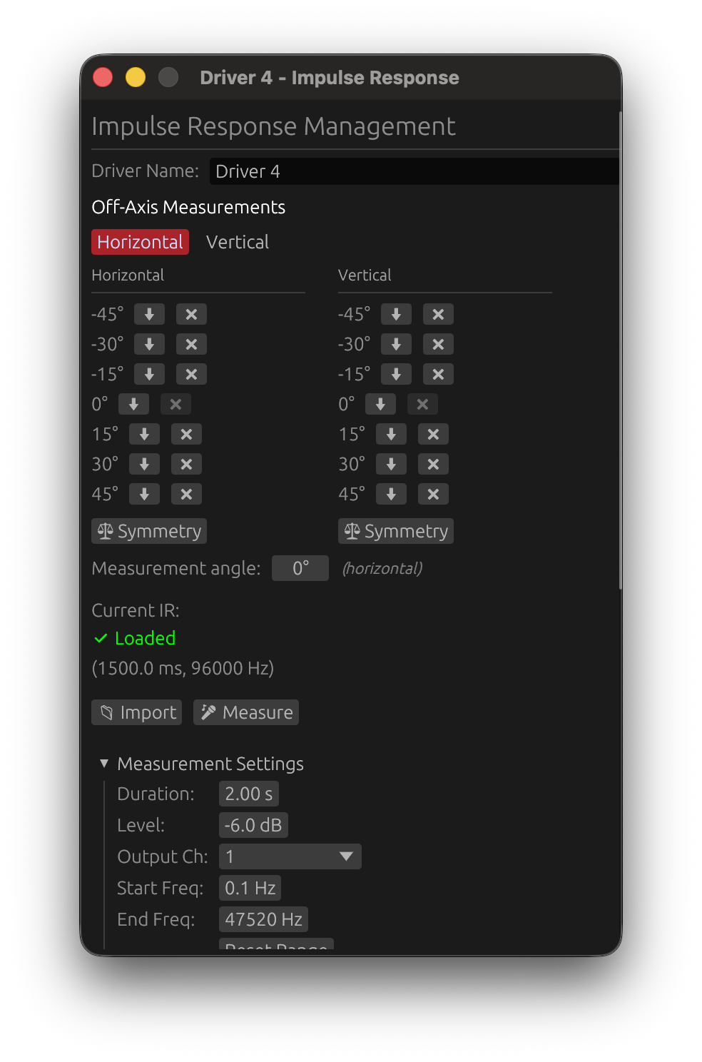
Accessing IR Management
Loudspeaker Design Mode:
- To open: Driver → Manage IR
- Purpose: Import, capture, and process driver impulse responses at multiple angles
Room Calibration Mode:
- To open: Measurements → Manage IR
- Purpose: Capture IR at a given in room position
Driver/Measurement Name
Manually enter a descriptive name for the impulse response.
- Label: “Driver Name” (Loudspeaker Design) or “Measurement Name” (Room Calibration)
- Purpose: Identify IRs in project and exports
- Persistence: Names are saved with the project
- Optional: Empty names default to “Driver X” or “Measurement X”
- Best practice: Use descriptive names like “Woofer_Left”, “Tweeter_RefXYZ”, “Position_Center”
Capturing IR
Button: 🎤 Measure
Triggers a measurement sweep with the configured parameters to capture the impulse response.
Features:
- Exponential sine sweep generation with configurable parameters
- Automatic harmonic distortion analysis (THD)
- Timing reference support for multi-driver measurements
For complete documentation on sweep parameters, driver protection, measurement workflow, and best practices, see Sweep Measurements.
Off-Axis Measurements 🔒
Available in: Loudspeaker Design mode only License required: Valid LinFIR license needed for off-axis measurements
Overview
Off-axis measurements enable directivity analysis by capturing impulse responses at different horizontal and vertical angles. These measurements are essential for understanding speaker radiation patterns and optimizing crossover design for consistent off-axis response.
Measurement Organization
Measurements are displayed in two columns:
-
Horizontal column: Measurements with vertical angle = 0°, varying horizontal angle
- Example: -90°, -60°, -30°, 0°, +30°, +60°, +90°
-
Vertical column: Measurements with horizontal angle = 0°, varying vertical angle
- Example: -60°, -40°, -20°, 0°, +20°, +40°, +60°
On-axis reference: The (0°, 0°) measurement appears in both columns.
Axis Selection
Before importing or capturing an off-axis measurement, select the measurement axis:
- Horizontal button: Measurements along horizontal axis (left/right)
- Vertical button: Measurements along vertical axis (up/down)
The selected axis determines whether the angle applies to horizontal or vertical position.
Measurement Angle
Field: “Measurement angle” Range: -180° to +180° Indicates: Angle for next import or capture operation
How it works:
- If Horizontal axis selected: angle applies to horizontal position (vertical = 0°)
- If Vertical axis selected: angle applies to vertical position (horizontal = 0°)
- The field shows which axis is active: “(horizontal)” or “(vertical)”
Restrictions:
- Disabled until on-axis (0°, 0°) measurement exists
- Requires valid LinFIR license
- Must import on-axis measurement first before adding off-axis angles
Per-Measurement Actions
Each measurement in the table has two action buttons:
Export Button (⬇)
Click to export this specific measurement:
- Opens export format dialog
- Choose WAV or TXT format
- Option to include distortion metadata
- File is saved with angle suffix (e.g.,
Driver1_v0h30.wav,Driver1_v-15h0.wav)
Delete Button (❌)
Remove a measurement from the driver:
- Off-axis measurements: Can be deleted freely
- On-axis (0°, 0°) measurement: Can only be deleted if all off-axis measurements are removed first
- This restriction exists because the on-axis measurement serves as the reference for all filter calculations
Tooltip guidance:
- Enabled: “Delete measurement”
- Disabled: “Delete all off-axis measurements first”
Export All Button
Button: ⬇ Export All Location: Above “Measurement angle” field Purpose: Export all measurements in a single operation
How it works:
- Click “⬇ Export All”
- Select output directory in file dialog
- All measurements are exported as WAV files
- Files use consistent naming:
DriverName_v{vertical}h{horizontal}.wav
File naming examples:
- On-axis:
Driver 1_v0h0.wav - Horizontal +30°:
Driver 1_v0h30.wav - Vertical -15°:
Driver 1_v-15h0.wav - Horizontal -45°:
Driver 1_v0h-45.wav
Format:
- All files exported as WAV (32-bit float, mono)
- Sample rate matches original measurement or importation sample rate
- Distortion metadata option applies to all files
- No individual format selection (always WAV)
Benefits:
- Fast export of complete measurement sets
- Consistent naming for re-import or external processing
- Files can be re-imported via batch import with automatic angle detection
Use cases:
- Archiving complete measurement sets
- Sharing measurements with collaborators
- Processing measurements in external tools (FIR Designer, Matlab, etc.)
Symmetry Tool
Button: ⚖ Symmetry Location: Below each column Purpose: Automatically duplicate measurements to opposite angles
How it works:
- Horizontal Symmetry: If you have +30°, creates -30° by mirroring the measurement
- Vertical Symmetry: If you have +20°, creates -20° by mirroring the measurement
Use case: Save measurement time by capturing one side and mirroring to the other side, assuming the speaker has symmetric radiation.
Workflow for Off-Axis Measurements
- Import or capture on-axis measurement (0°, 0°) first
- Select axis (Horizontal or Vertical)
- Set measurement angle (e.g., +30°)
- Import file or capture measurement
- Repeat for additional angles
- Use Symmetry tool to fill opposite angles (optional)
- Analyze directivity patterns in main application graphs
🔄 Automated workflow: If you have a motorized turntable (Pololu Tic or GRBL/Arduino), use the ▶ Scan button to rotate and measure all angles automatically. See Auto-Scan with a Rotation Table and Rotation Table Settings.
Import from File
Load impulse responses from external files.
LinFIR works internally with impulse responses (IRs). All imported files are ultimately converted to an IR before being used for filter design. Two import paths exist:
- Direct IR formats (WAV, TXT, TMD): Files already contain time-domain impulse response samples. They are resampled to the project sample rate and loaded directly.
- Frequency-domain format (FRD): Files contain frequency response data (magnitude + phase). LinFIR reconstructs an impulse response via the FRD to IR Converter window before proceeding.
Supported Formats
WAV Files
- Channels: Mono or stereo (left channel used for stereo files)
- Bit depth: 16-bit, 24-bit, or 32-bit PCM
- Automatic resampling: The IR is resampled to match the project sample rate for processing. The original samples are preserved internally at their native rate, so changing the project sample rate later does not cause quality loss from successive resamplings. This is handled transparently in the background.
With distortion metadata:
- If WAV contains custom ‘dist’ chunk (exported from LinFIR with “Include dist.” option)
- Enables THD (Total Harmonic Distortion) computation
Without distortion metadata:
- Standard WAV import
- Only practical/cropped IR available
- THD computation not available
TXT Files
Plain text files containing impulse response samples, one value per line or space/comma-separated. LinFIR auto-detects this format.
Note: .txt files containing FRD-formatted data (3 columns: frequency, magnitude, phase) are automatically detected and processed as FRD files (see FRD Files section below).
TMD Files
MATAA (Mat’s Audio Analyzer) time-domain data format. Each line encodes a sample with its timestamp, allowing the sample rate to be derived from the data itself.
- Format: Two-column text file (time in seconds, amplitude)
- Comments: Lines starting with
*are metadata/comments - Sample rate: Inferred from the time intervals between samples. If the result is within 1% of a standard rate (44.1, 48, 88.2, 96, 176.4, 192, 384 kHz, etc.), LinFIR snaps to that exact rate to correct for the systematic sample rate error introduced by limited timestamp precision.
- Timestamp precision: Timestamps must have enough decimal places for accurate sample rate inference (e.g. 9 digits for 96 kHz). Insufficient precision can produce a slightly off sample rate that will still be corrected if it falls within the 1% snapping tolerance.
- Precision: Full floating-point precision (no bit-depth limitations)
Example TMD file:
* TMD data written by MATAA
* Measurement description
0.000000000	0.000000
0.000020833	0.125000
0.000041667	0.850000
...
CLIO Files
Time-domain impulse response exports from CLIO (Audiomatica) measurement software. These are plain .txt files with three columns.
- Format: Text file with a header row followed by data rows
- Column 1 —
Time[s]: sample timestamp in seconds - Column 2 —
Real[Pa]: signal amplitude (used as the IR) - Column 3 —
Imag[Pa]: imaginary part (ignored by LinFIR)
- Column 1 —
- Header line: the first non-empty line must start with
Time(case-insensitive) - Sample rate: inferred from the time intervals between samples, then snapped to the nearest standard rate within 1% tolerance (same algorithm as TMD)
- Precision: full floating-point precision
Example CLIO file:
Time[s]         Real[Pa]        Imag[Pa]
0.000000E+00    -4.790139E-03   -4.583853E-10
2.083333E-05     4.526122E-03   -8.076313E-10
4.166667E-05     3.454284E-04    1.007265E-10
...
FRD Files
Frequency response data files (commonly exported by REW, VituixCAD, or provided by manufacturers). These files do not contain an impulse response directly—LinFIR reconstructs one via the FRD to IR Converter window (see dedicated section below).
Format:
- 3 columns per line: Frequency (Hz), Magnitude (dB), Phase (degrees)
- Text-based, space or tab delimited
- Can use either
.frdextension or.txtextension (auto-detected)
Processing:
- Automatic interpolation to required frequency points using PCHIP (Piecewise Cubic Hermite Interpolating Polynomial)
- Configurable magnitude extrapolation for DC and high-frequency regions
- Phase handling with group delay compensation
Extrapolation Modes:
When importing FRD files, LinFIR opens the FRD to IR Converter window with the following extrapolation controls:
-
DC Extrapolation: Controls how magnitude is extended below the lowest measured frequency
- Constant: Flat extrapolation (holds the lowest measured value)
- Roll-off: Applies a 12 dB/octave high-pass roll-off for realistic loudspeaker behavior
- Default: Roll-off
-
High Frequency Extrapolation: Controls how magnitude is extended above the highest measured frequency toward Nyquist
- Constant: Flat extrapolation (holds the highest measured value)
- Roll-off: Applies a 12 dB/octave low-pass roll-off, automatically compensates for upward slopes
- Default: Constant
Benefits of Roll-off mode:
- More realistic impulse responses from incomplete FRD data
- DC roll-off mimics natural loudspeaker low-frequency limitations
- HF roll-off prevents artifacts from measurements that don’t extend to Nyquist
- Adaptive: compensates for incorrect slope trends in measured data
Important notes:
- FRD files are sparse (often logarithmically spaced frequency points)
- Requires complex interpolation, potentially introducing artifacts
- Generally do not contain the time of flight required to properly time align drivers
- Recommendation: Prefer importing impulse responses (WAV) whenever possible
Automatic Noise Truncation
Once an impulse response has been imported or reconstructed (from any format), LinFIR automatically truncates it to optimize file length and processing performance. This is an internal post-processing step applied uniformly to all IR data before it is stored in the project.
Truncation Algorithm:
- Peak detection: Locates the main impulse peak (maximum absolute value in the IR)
- 5-second limit: Truncates the IR to 5 seconds maximum after the peak
- Corresponds to approximately 1.7 km acoustic distance
- Sufficient for capturing full decay in most practical scenarios
- Noise threshold: Removes trailing samples below 0.1% of peak amplitude
- Adaptive threshold based on the actual signal level
- Eliminates noise floor without affecting useful signal
- Minimum duration: Always preserves at least 1.0 seconds of the IR
- Ensures sufficient data for low-frequency analysis
Benefits:
- Reduces processing load for FFT operations and convolutions
- Decreases file sizes for project saving and export
- Removes unnecessary noise floor that doesn’t contribute to filter design
What gets removed:
- Excessive silence beyond 5 seconds after the main impulse
- Noise floor below the 0.1% threshold (≈ -60 dB relative to peak)
- Applies to both anechoic and in-room measurements
What is preserved:
- The complete main impulse and initial decay
- At least 1.0 seconds of IR data regardless of noise level
- All frequency content relevant for crossover design
- Sufficient time-domain information for phase analysis
Impulse Response Timing Requirements
Peak delay limit: LinFIR rejects impulse responses where the main peak is located more than 200 ms after the start of the file.
Why this limit exists:
LinFIR performs extensive signal processing operations—FFT transformations, convolutions, resampling, and real-time filter preview—that must remain responsive. These operations scale with impulse response length, and excessive zero padding before the actual signal significantly impacts performance without adding useful information.
Physical context:
A 200 ms delay corresponds to approximately 68 meters of acoustic travel distance. In practical loudspeaker measurement and room calibration scenarios, such excessive delays indicate that no timing reference method was used during capture (loopback trigger, electrical reference, or pre-alignment in the measurement software).
Impact on workflow:
Without proper timing reference, relative time alignment between drivers becomes unreliable, as the arbitrary delays vary unpredictably between measurements. This compromises crossover phase coherence and summation accuracy—core functions of LinFIR.
Best practice:
When capturing impulse responses, use measurement software that provides:
- Loopback triggering (audio interface output → input reference)
- Electrical reference triggering (synchronized start)
- Pre-alignment features that position the IR peak near the beginning of the recording
These methods ensure minimal file length while preserving the precise time-of-flight information needed for accurate driver alignment and filter design.
If your measurement contains a valid signal buried in initial silence, pre-process the file to remove leading zeros before importing into LinFIR.
Import Workflow
- Click “📁 Import” button
- Select WAV, TXT or FRD file
- File is automatically detected and processed:
- WAV: Resampled to project sample rate, metadata extracted
- TXT (impulse samples): Either auto-imported (with metadata) or user prompted for sample rate
- TXT/FRD (frequency data): Opens FRD to IR Converter window
- IR appears in impulse response graph
- Manually enter IR name in text field
- Apply windowing if necessary (see Time Windowing section)
Special case for FRD files: When importing .frd or FRD-formatted .txt files, the FRD to IR Converter window opens automatically. See the dedicated section below for details.
⚠️ Display Mode Check: If the imported impulse response does not appear in the graphs, verify that Drivers/Measurements display mode is selected in the graph toolbar (not FIR, IIR, or FIR+IIR modes which only show filter responses). The graph title and legend clearly indicate which mode is active.
Batch Import of Multiple Measurements
Available in: Loudspeaker Design mode (off-axis measurements) License required: Valid LinFIR license needed for off-axis measurements
Overview
Batch import enables importing multiple measurement files simultaneously with automatic angle detection from filenames. This significantly speeds up the workflow when importing multi-angle measurement sets from tools like VituixCAD, ARTA, or REW.
Filename Angle Parsing
LinFIR automatically detects measurement angles from filenames using conventions from other measurement software.
Important: Angle patterns must be at the end of the filename (before extension). If the axis marker (h/v) has a prefix format (like h30), it must not be preceded by a letter. This prevents false detection in cases like “Driverh30” while allowing “SIG270-4h30” or “Driver 2_h30”.
Format with single axis specification (H = Horizontal, V = Vertical):
H30,h30,H-20→ Horizontal axis, angles: +30°, +30°, -20°V15,v15,V-45→ Vertical axis, angles: +15°, +15°, -45°30H,30h,-20H→ Horizontal axis, angles: +30°, +30°, -20°15V,15v,-45V→ Vertical axis, angles: +15°, +15°, -45°
Format without axis (@ marker):
@30,@-20,Tweeter@15→ Angle detected, axis must be specified by user- When files use @ notation, a dialog prompts you to select Horizontal or Vertical axis
MF 2D format (both H and V in filename):
v0h30,V0H30,v000h030→ Horizontal +30° (horizontal plane: V=0)v30h0,V30H0,v030h000→ Vertical +30° (vertical plane: H=0)h30v0,H30V0,h030v000→ Horizontal +30° (order-independent)h0v30,H0V30,h00v030→ Vertical +30° (order-independent)v0h0,V0H0,v000h000→ On-axis (0°, 0°)v30h50→ Rejected (out-of-plane measurement)
Note: Leading zeros are supported (e.g., 030 = 30)
Note on MF 2D format: Only measurements in a plane are accepted (one angle must be 0). Files with both H and V non-zero are ignored as they represent oblique measurements that can’t be represented in LinFIR’s horizontal/vertical coordinate system. The order of h/v doesn’t matter.
Examples of valid filenames:
Tweeter_h0.wav→ On-axis (0°, 0°)Tweeter_h30.wav→ Horizontal +30°Tweeter_v-20.frd→ Vertical -20°Woofer@15.txt→ Angle +15° (user selects axis)measurement_30h.wav→ Horizontal +30°Left_-45v.frd→ Vertical -45°Driver_v0h45.frd→ Horizontal +45° (MF 2D format)Tweeter_v20h0.txt→ Vertical +20° (MF 2D format)SIG270-4h30.frd→ Horizontal +30° (number before axis letter is OK)SIG270-4v0h30.frd→ Horizontal +30° (MF 2D with number prefix)
Examples of rejected filenames:
Driverh30.wav→ Rejected (letter “r” directly before “h”)Testh30v0.frd→ Rejected (letter “t” directly before “h”)
Files without angle markers:
- Imported as on-axis (0°, 0°) measurement
- You can still manually set the angle before importing if needed
Batch Import Workflow
1. Multi-File Selection
- Click “📁 Import” button
- Select multiple files in the file dialog (Ctrl+Click or Shift+Click)
- Click Open
2. Automatic Processing
LinFIR automatically analyzes all selected files:
If all files have explicit axis (H/V in filename):
- Files are processed immediately
- Each file imported at the angle specified in its filename
- No user interaction needed
If files use @ notation (ambiguous axis):
- Axis Selection Dialog appears
- Select either Horizontal or Vertical axis
- Click Continue
- Selected axis applies to all @ files in the batch
3. FRD Converter Integration
If the batch includes FRD files:
- LinFIR opens the FRD Converter for the on-axis FRD file (if present)
- Configure conversion parameters (sample rate, delay, extrapolation modes)
- Click “Use This Impulse Response”
- All remaining FRD files automatically use the same parameters
- No need to configure each file individually
How it works:
- Parameters are configured using the on-axis measurement (0°, 0°)
- Same delay and extrapolation settings applied to all off-axis FRD files
- Ensures consistent conversion across the measurement set
⚠️ Important Limitation - Missing Relative Time Delays:
FRD files contain frequency response data only (magnitude and phase) without encoding the relative time delays between different measurement angles. When importing multiple FRD files at different angles, all files use the same delay parameter configured on the on-axis measurement.
Why this matters for off-axis measurements:
In real loudspeakers, off-axis measurements have different acoustic path lengths and interference patterns compared to on-axis:
- Sound from tweeter and woofer arrives at different relative times depending on measurement angle
- These time differences create frequency-dependent interference (comb filtering)
- Proper time alignment between drivers varies with angle
Consequence:
- Batch-imported FRD files will have identical relative timing at all angles
- Phase relationships between drivers won’t reflect actual acoustic behavior
- Directivity analysis and crossover optimization will be inaccurate
- Simulated off-axis response won’t match real-world interference patterns
Recommendation:
- Prefer WAV impulse response files for multi-angle measurements whenever possible
- WAV files preserve the actual time-of-flight at each angle
- Only use FRD batch import for preliminary analysis or when WAV files aren’t available
- If using FRD files, be aware that off-axis crossover behavior won’t be accurately modeled
Valid use cases for batch FRD import:
- Quick magnitude response comparison across angles
- Preliminary directivity visualization
- Single-driver systems where relative timing isn’t critical
- When no impulse response measurements are available
Practical Example
Scenario: You have a set of horizontal measurements exported from REW:
Tweeter_h0.frd
Tweeter_h15.frd
Tweeter_h30.frd
Tweeter_h45.frd
Tweeter_h60.frd
Workflow:
- Select all 5 files in file dialog
- FRD Converter opens for
Tweeter_H0.frd(on-axis) - Set sample rate to 96000 Hz, delay to 5 ms
- Choose DC extrapolation: Roll-off
- Click “Use This Impulse Response”
- Files
H15,H30,H45,H60automatically converted with same settings - All 5 measurements appear in the horizontal column
Result:
- All angles have same delay (5 ms) configured on on-axis measurement
- ⚠️ Relative time-of-flight differences between angles are lost
- For accurate crossover modeling, prefer WAV impulse response files
Limitations
- Batch import only works with files having consistent format (all WAV, all FRD, or mixed)
- Files must follow supported angle naming conventions
- On-axis measurement (0°, 0°) should be included when importing FRD files for optimal parameter configuration
- If mixing WAV and FRD formats, FRD files must include on-axis or parameters will use defaults
- FRD files don’t preserve relative time delays between angles—prefer WAV files for multi-angle measurements
Tips
Consistent naming convention:
- Use descriptive base names:
Tweeter_h30.wavinstead of justh30.wav - Include driver name in filename for easier identification
- Use lowercase h/v for consistency with LinFIR exports
- MF 2D format is order-independent:
v0h30=h30v0
Large measurement sets:
- Import horizontal and vertical measurements separately if you have both
- Use Symmetry tool after batch import to fill missing opposite angles
- Verify measurement table after import to ensure correct angle assignment
FRD files:
- ⚠️ Not recommended for off-axis measurements (missing relative time delays)
- Always include on-axis (H0 or V0) measurement in batch for parameter reference
- Configure extrapolation modes carefully for first file—settings propagate to all
- Verify impulse response quality after batch conversion
- Consider this a preliminary workflow—prefer WAV files for accurate directivity analysis
Recommended format priority:
- WAV files: Best option—preserves all timing information
- TXT with metadata: Acceptable if exported from LinFIR
- FRD files: Only for magnitude analysis—timing not preserved
FRD to IR Converter
When importing FRD files, LinFIR opens a dedicated conversion window with advanced tools for interpolation, visualization, and quality assessment.
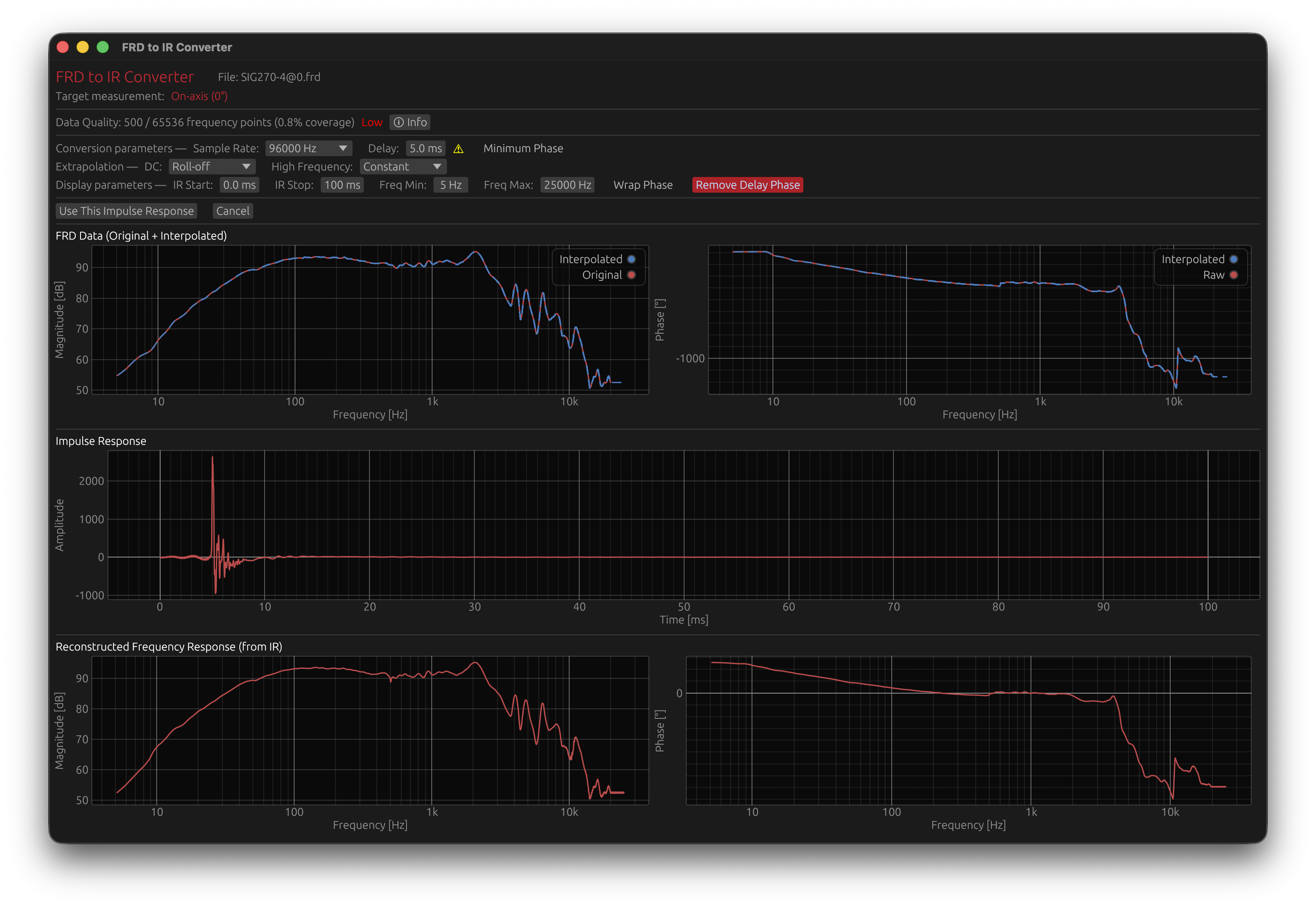
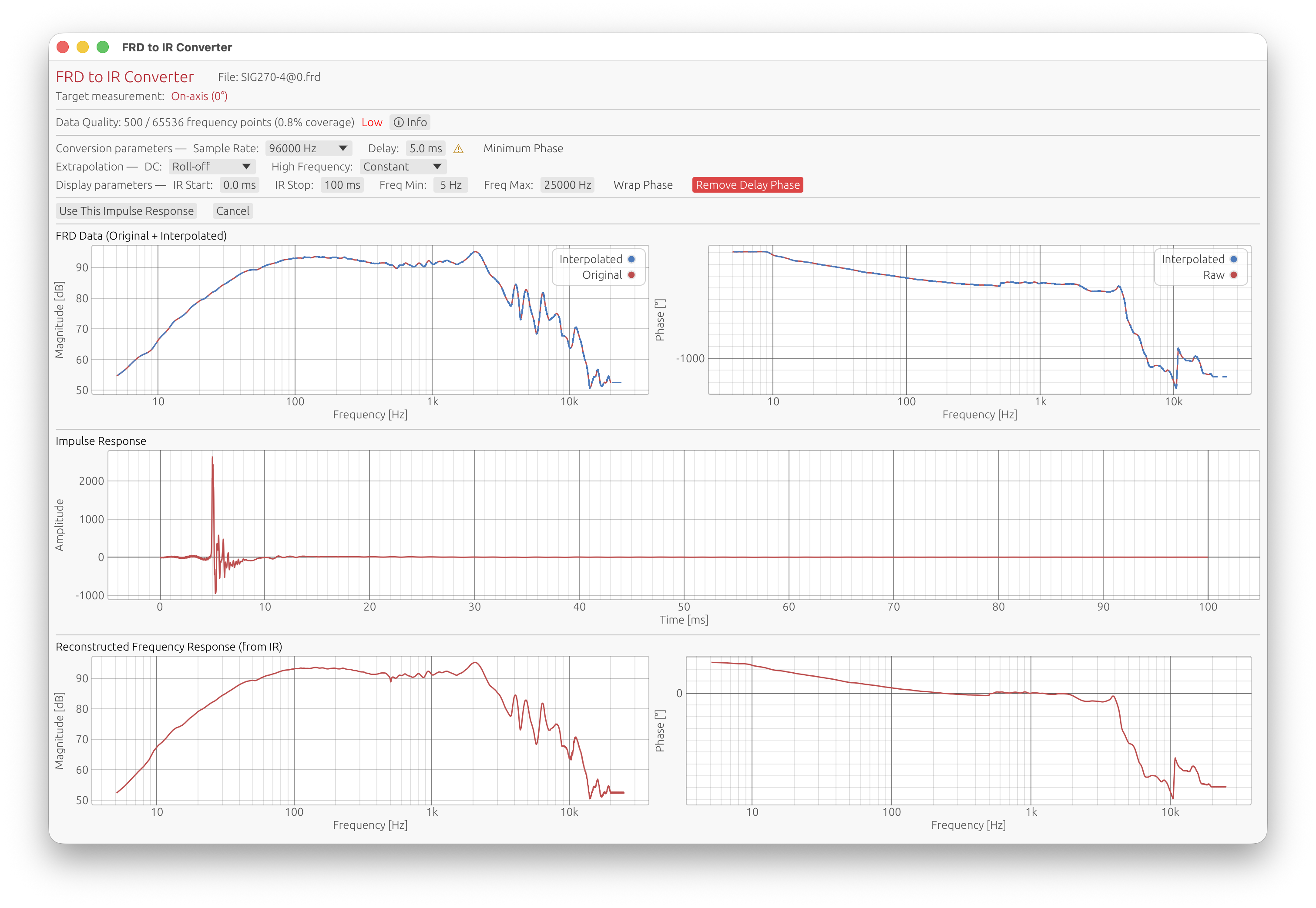
Overview
The FRD to IR Converter transforms sparse frequency-domain data into time-domain impulse responses using sophisticated interpolation and extrapolation techniques. It provides real-time visualization and quality metrics to help you assess the conversion quality.
Conversion Parameters
Sample Rate
Options: 44.1 kHz, 48 kHz, 88.2 kHz, 96 kHz, 176.4 kHz, 192 kHz Default: 96 kHz
Target sampling frequency for the resulting impulse response.
Considerations:
- Higher sample rates provide better frequency resolution
- Must match or exceed your project’s sample rate
- FRD data is interpolated to fill all frequency bins from DC up to Nyquist
Delay Compensation
Range: 0.0 to 100.0 ms Default: 5.0 ms
Time offset applied to the impulse response to allow for pre-ringing visualization and processing.
Purpose:
- Provides time buffer before the main impulse
- Essential when FRD data contains non-minimum phase characteristics
- Allows visualization of pre-ringing artifacts
Warning indicator: If pre-ringing duration exceeds the delay setting, a warning appears suggesting either:
- Increase delay to accommodate pre-ringing
- Enable Minimum Phase transformation
Minimum Phase Transformation
Default: Disabled
Applies Hilbert transform to convert the impulse response to minimum phase, eliminating all pre-ringing.
When to use:
- FRD data shows significant pre-ringing (> 5% energy before peak)
- Phase data is corrupted, smoothed, or contains wrapping errors
- You need a causal, physically realizable impulse response
- Time-domain alignment is critical
Effects:
- Removes all energy before the main peak
- Preserves magnitude response
- Changes phase response to minimum phase equivalent
- Results in a causal system (no pre-ringing)
Note: Pre-ringing in FRD-derived impulses is often an artifact of measurement or file creation, not a physical characteristic of the device.
DC Extrapolation
Modes: Constant, Roll-off Default: Roll-off
Controls how magnitude is extended below the lowest measured frequency toward DC (0 Hz).
Constant mode:
- Flat extrapolation using the lowest measured value
- Use when FRD data already reaches very low frequencies
Roll-off mode (recommended):
- Applies 12 dB/octave high-pass characteristic
- Mimics natural loudspeaker low-frequency roll-off
- More physically realistic for incomplete low-frequency data
High Frequency Extrapolation
Modes: Constant, Roll-off Default: Constant
Controls how magnitude is extended above the highest measured frequency toward Nyquist.
Constant mode (recommended):
- Flat extrapolation using the highest measured value
- Maintains adequate signal level to Nyquist
- Minimizes noise amplification
Roll-off mode:
- Applies 12 dB/octave low-pass characteristic
- Automatically compensates for upward slope trends
- Use when FRD data shows unrealistic high-frequency behavior
Driver Offset Compensation
The FRD to IR Converter provides Driver Offset controls to compensate for the physical displacement of the driver relative to the reference point (typically the front baffle center or another driver).
Parameters:
- X (Horizontal): Driver offset in the horizontal direction, in millimeters
- Y (Vertical): Driver offset in the vertical direction, in millimeters
- Located below the Extrapolation controls in the converter window
Coordinate System and Geometry:
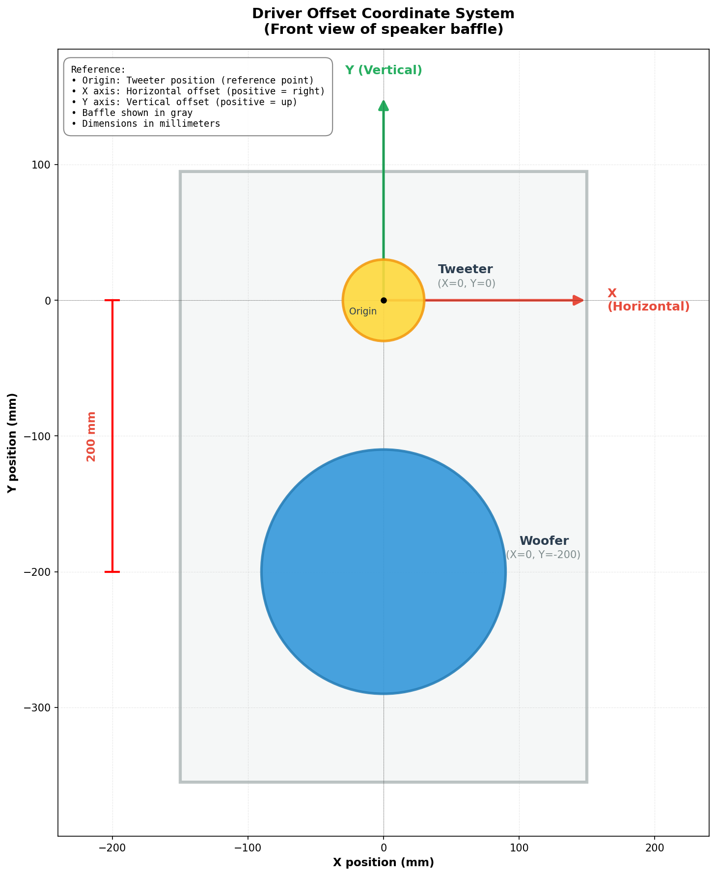
Reference Point (Origin):
The reference point (X=0, Y=0) represents the desired acoustic axis of the loudspeaker system. In the diagram example:
- The tweeter is positioned at the origin (0, 0) — it defines the acoustic axis
- The woofer is offset by -200 mm vertically (0, -200)
Note for designers: The choice of origin is not necessarily the center of a driver — it’s an engineering decision. You could choose:
- The acoustic center of a specific driver (as shown in the example)
- A point between drivers (e.g., midway between tweeter and woofer)
- Any other reference point that makes sense for your design goals
What matters is consistency: all driver offsets are measured relative to this chosen origin.
Important: For off-axis measurements, only a driver with offset (woofer in the example) will have geometric delay applied. A driver at the origin (tweeter in the example) has no delay added or subtracted for off-axis angles — it remains the reference. This delay difference is then used to calculate interference patterns between drivers at off-axis angles.
How it works:
The driver offset introduces an additional geometric delay for off-axis measurements, calculated using the far-field approximation with Euclidean distance:
$$\Delta t = \frac{\sqrt{(x \cdot \sin\theta)^2 + (y \cdot \sin\varphi)^2}}{c}$$
Where:
- \(x\) = horizontal driver offset (mm)
- \(y\) = vertical driver offset (mm)
- \(\theta\) = horizontal measurement angle (degrees)
- \(\varphi\) = vertical measurement angle (degrees)
- \(c\) = speed of sound ≈ 343,000 mm/s
In practice (measurements in a single plane):
Since LinFIR only supports measurements in the horizontal plane (\(\theta \neq 0\), \(\varphi = 0\)) or vertical plane (\(\theta = 0\), \(\varphi \neq 0\)), the formula simplifies:
- Horizontal plane: \(\Delta t = \frac{x \cdot \sin\theta}{c}\) (only x offset matters)
- Vertical plane: \(\Delta t = \frac{y \cdot \sin\varphi}{c}\) (only y offset matters)
The Euclidean formula is used in the code to be mathematically correct and future-proof should oblique measurements be supported.
This geometric delay is added to the user-configured delay before converting the FRD data to an impulse response.
Example:
- Tweeter at origin (0, 0): no geometric delay applied at any angle
- Woofer offset: X = 0 mm, Y = -200 mm
- Measurement at vertical -30° (30° below axis)
- Geometric delay for woofer: \(200 \times \sin(30°)/343000 \approx 0.291\) ms
- This delay difference creates the correct interference pattern between tweeter and woofer at -30°
Purpose and Far-Field Approximation:
⚠️ Purpose: Driver offsets are used to predict far-field interference patterns between drivers when the listener is in the far field (listening distance >> driver spacing).
Key insight: Since typical FRD data has its phase recalculated (constant delay removed), the original measurement conditions don’t matter. What matters is modeling the acoustic geometry at the listening position.
When to use driver offsets:
- Listening distance ≥ 10× driver spacing (far-field condition for the listener)
- Example: For drivers spaced 200 mm apart, listener at ≥ 2 meters
- Typical home listening (2-4m) and studio monitoring (2-3m) scenarios
- Predicting directivity and off-axis response in real-world use
Geometric assumption:
The formula assumes acoustic rays are parallel at the listening position:
- Valid when listener distance >> driver spacing
- Path difference depends only on driver offset and angle
Near-field listening considerations:
For close listening distances (< 1m), the parallel ray approximation becomes less accurate for the direct sound, and the predicted response will deviate more from reality as you get closer to the drivers.
However, the approximation remains valid for the reflected sound field since walls, floor, and ceiling are typically far enough that the acoustic path length is much larger than driver spacing. This is important because off-axis directivity affects how sound interacts with room boundaries.
Best practice:
- Use driver offsets in most scenarios, including near-field listening
- The approximation is excellent for far-field listening (≥ 2m)
- For near-field use (< 1m), understand that direct sound predictions will be approximate, but reflected field modeling remains valid
- Leaving offsets at 0 mm corresponds to a coaxial driver configuration (all drivers at the same point)
Display Parameters
These parameters control visualization only and do not affect the conversion.
IR Start / Stop Time
Range: 0.0 ms to impulse duration Purpose: Zoom into specific time region of the impulse response graph
Useful for examining:
- Pre-ringing characteristics
- Main peak detail
Frequency Min / Max
Range: 1 Hz to 48000 Hz Purpose: Set frequency range for magnitude and phase graphs
Allows focusing on:
- Specific frequency bands of interest
- Problem areas in the response
- Comparison between original and interpolated data
Wrap Phase
Default: Disabled
Toggles between wrapped (-180° to +180°) and unwrapped phase display.
Wrapped:
- Phase limited to -180° to +180° range
- Shows discontinuities at ±180° boundaries
- Familiar format for some users
Unwrapped:
- Continuous phase (can exceed ±180°)
- Shows true phase accumulation
- Better for assessing group delay trends
Remove Delay Phase
Default: Disabled
Removes the linear phase component corresponding to the delay setting.
When enabled:
- Subtracts linear phase = -360° × f × delay
- Reveals underlying phase structure
- Useful for comparing final phase response with the original one
Data Quality Assessment
The converter displays comprehensive quality metrics to help you evaluate the FRD data.
Coverage Metric
Format: “X / Y frequency points (Z% coverage)”
- X: Number of frequency points in FRD file (within 0 Hz to Nyquist)
- Y: Expected number of points for complete FFT coverage
- Z: Coverage percentage = (X / Y) × 100
Quality indicators:
- ✅ Good (≥ 50%): Green - Sufficient data density
- ⚠️ Moderate (20-50%): Yellow - Acceptable but sparse
- ❌ Low (< 20%): Red - Very sparse, heavy interpolation required
FFT bin calculation: Based on sample rate and FFT size (4× next power of 2)
Info Button - Detailed Diagnostics
Click the ℹ Info button to open the Data Quality Information window with detailed analysis.
Missing DC (0 Hz):
- Impact: Low-frequency extrapolation required
- Consequence: Uncertainty in bass response below lowest measured frequency
- Solution: Use Roll-off extrapolation for DC
Missing Nyquist Data:
- Impact: High-frequency extrapolation required
- Consequence: Uncertainty in high-frequency response
- Recommended: FRD should extend to at least Nyquist frequency
Sparse Frequency Data:
- Threshold: < 50% coverage
- Impact: Heavy interpolation between measured points
- Risk: Artifacts from PCHIP interpolation of widely-spaced points
- Note: Shows exact percentage of missing data points
Pre-ringing Detection:
Analyzed automatically after conversion. Three severity levels:
-
Minor (0.1% - 0.5% energy before peak):
- Blue indicator
- May indicate slight phase smoothing or measurement artifacts
- Usually acceptable for most applications
-
Moderate (0.5% - 1.0% energy before peak):
- Yellow/Orange warning
- Phase data likely smoothed or contains wrapping errors
- Consider minimum phase transformation
-
Significant (≥ 1.0% energy before peak):
- Red warning
- Severe phase corruption or non-physical characteristics
- Strongly recommended: Enable Minimum Phase transformation
- Will affect transient response and phase correction accuracy
Pre-ring duration: Time span from first significant energy to main peak
Physical interpretation: Real loudspeakers cannot produce energy before the stimulus arrives. Pre-ringing in FRD files indicates:
- Phase data smoothing in measurement software
- Phase wrapping/unwrapping errors
- File export artifacts
- Non-minimum phase processing applied to data
Impact Warnings
The Data Quality Information window provides context on how issues affect the conversion:
Missing Data Effects:
- Artifacts in reconstructed impulse response
- Estimated information through interpolation/extrapolation
- Final impulse may not fully represent original system
Best Practices for FRD Files:
- Include DC (0 Hz) measurement point
- Extend data to at least Nyquist frequency
- Aim for > 50% frequency coverage
- Prefer linear frequency spacing over logarithmic
- Avoid phase smoothing in export settings
Time-Domain Preference:
The converter emphasizes: When possible, import impulse responses (WAV files) instead of FRD.
Advantages of time-domain data:
- No interpolation artifacts
- Preserves time-of-flight information (with proper timing reference)
- Essential for proper driver alignment in crossover design
- Natural representation of system behavior
FRD limitations for crossover design:
- Often lacks time-of-flight data
- Driver motors may not be coplanar
- Diaphragm geometry affects acoustic center
- Horn loading adds group delay
- Relative delays between drivers are essential
Visualization Graphs
The converter displays three synchronized graphs:
1. FRD Data (Original + Interpolated):
- Left: Magnitude response
- Right: Phase response
- Red curve: Original FRD measurements
- Dashed blue curve: PCHIP interpolated curve
2. Impulse Response:
- Reconstructed time-domain impulse
- Zoom using IR Start/Stop controls
- Shows pre-ringing and overall IR structure
3. Reconstructed Frequency Response:
- Left: Magnitude computed from impulse via FFT
- Right: Phase computed from impulse via FFT
- Validation: Should closely match interpolated FRD (with Remove Delay Phase button enabled)
- Differences indicate reconstruction issues
Workflow
- Import FRD file - Converter window opens automatically
- Review quality metrics - Check coverage and warnings
- Adjust extrapolation - Set DC and HF modes as needed
- Set sample rate - Match or exceed project sample rate
- Configure delay - Ensure adequate pre-ringing buffer
- Enable minimum phase - If pre-ringing > 1% or phase corrupted
- Inspect graphs - Verify interpolation and reconstruction quality
- Click “Use This Impulse Response” - Apply to selected measurement angle
The converted impulse is automatically stored in the driver’s measurement at the specified horizontal/vertical angle.
Microphone Calibration
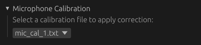
Apply frequency response and sensitivity calibration corrections for your measurement microphone.
Overview
Each driver or room measurement can be assigned a microphone calibration that compensates for:
- Frequency response deviation from ideal flat response
- Sensitivity factor (dB conversion from microphone output to SPL)
Calibration management:
- Calibration files are managed in Settings → Mic Calibration (see Settings → Mic Calibration)
- Default calibration can be set for new drivers
- Each driver/measurement can use a different calibration or none at all
Calibration Dropdown
Location: Below the Driver/Measurement Name field
Options:
- None: No calibration applied (use for reference microphones or pre-calibrated measurements)
- [Calibration file names]: All imported calibration files from Settings → Mic Calibration
Behavior:
- Selection is saved with the project file
- Calibration data is stored in application settings, not in project files
- Changing the selection immediately recomputes the driver’s windowed IR and all filter responses
How Calibration is Applied
Processing pipeline:
- Measurement is imported and windowed (see Time Windowing)
- Microphone calibration correction applied (if selected)
- Minimum-phase FIR filter created from frequency response data
- Sensitivity factor (dB) applied as gain adjustment
- Frequencies below 5 Hz filtered out before processing
- Corrected IR used for all subsequent filtering (crossovers, correction filters, etc.)
Phase behavior:
- Correction uses minimum-phase reconstruction, affecting both magnitude and phase
- This is physically accurate for measurement microphones, which exhibit mainly minimum-phase behavior
Real-time updates:
- Calibration is recomputed whenever you change the windowing parameters
- Filter responses update automatically when you change calibration selection
When to Use Calibrations
Apply calibration when:
- Using consumer or measurement microphones with non-flat response
- You have calibration data from the manufacturer or third-party calibration service
- Measurements were taken with the same microphone used for the calibration file
Use “None” when:
- Measurements were taken with an already-flat reference microphone
- Importing measurements already compensated externally
Per-Driver vs. Default Calibration
Per-driver assignment (this window):
- Overrides any default set in Settings
- Useful when combining measurements from different microphones in one project
- Saved with the project file
Default calibration (Settings → Mic Calibration):
- Automatically applied to newly created drivers/measurements
- Does not affect existing drivers
- See Settings → Mic Calibration for configuration
Time Windowing
Isolate the direct sound from an impulse response and exclude reflections or noise.
Note: Time windowing is not available in Room Calibration mode. This is intentional: Room Calibration mode is designed to capture the full speaker-plus-room response, including reflections and room decay. Applying a time window would produce an anechoic-like impulse response — corrections derived from it would be wrong for the actual listening environment — what you hear is the direct sound from the speakers combined with all the reflections that follow, and the correction filters must account for that full response.

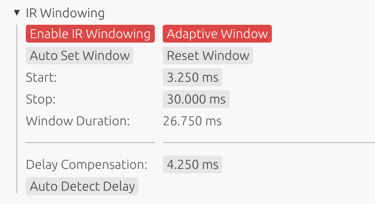
Parameters
Start Time
Beginning of the time window in milliseconds.
- Purpose: Remove pre-ringing or early noise
- Typical: 0.0 to 5.0 ms before main peak
- Effect: Sets the beginning of the extracted portion
Stop Time
End of the time window in milliseconds.
- Purpose: Exclude late reflections or room decay
- Typical: 5.0 to 100.0 ms after main peak
- Effect: Sets the end of the extracted portion
Duration Display
Wndow duration (Stop Time - Start Time).
Auto Set Window
Click “Auto Set Window” to automatically detect and configure optimal window boundaries.
How It Works:
The algorithm analyzes the on-axis measurement (0°, 0°) and automatically sets the start and stop times:
- Detect main peak: Locates the largest absolute amplitude in the impulse response
- Compute Hilbert envelope: Calculates the amplitude envelope for robust reflection detection
- Adaptive threshold: Adjusts detection sensitivity based on signal-to-noise ratio (3-8% of peak)
- Set start time: Places window start 3 ms before the main peak (clamped to 0.0 minimum)
- This margin accounts for off-axis measurements where the sound path may be shorter (gives a margin of ~1m)
- Prevents truncation of the direct sound in off-axis measurements
- Search for reflections: Scans the envelope for the first significant reflection/echo after the main peak:
- Must occur at least 3 ms after the main peak
- Must exceed the adaptive threshold
- Must be a local maximum in the envelope
- Set stop time: Places window stop 0.5 ms before the first detected reflection
If no significant reflection is detected, the stop time is set to the end of the search window or IR length.
Detection Method:
The algorithm uses Hilbert envelope analysis to detect reflections. This provides more robust detection than simple amplitude analysis by following the overall energy contour of the signal, making it less sensitive to oscillations within the waveform.
Window Margins:
- Start margin (3 ms): Ensures off-axis measurements are not truncated when rotating large loudspeakers. At the speed of sound (~343 m/s), 3 ms corresponds to approximately 1 meter of path length difference. During rotation, drivers may move closer to or further from the microphone—this margin provides sufficient safety for rotations of large cabinet.
- Stop margin (0.5 ms): Small margin before the detected reflection to avoid including the beginning of the echo.
Best Use Cases:
- ✅ Quasi-anechoic measurements: Ideal for measurements with clear, isolated reflections (e.g., outdoor, treated rooms, gated measurements)
- ✅ Controlled environments: Works well when the direct sound is clearly separated from reflections
- ✅ Multi-angle measurements: The 3ms start margin prevents truncation of off-axis measurements
- ✅ Time-saving: Quick initial window setup that can be manually refined if needed
Limitations:
- ❌ Reverberant environments: Not suitable for highly reflective rooms where reflections arrive continuously
- ❌ Dense reflection patterns: May not detect the first reflection correctly if multiple reflections arrive in quick succession
- ❌ Room measurements: For full-room measurements including reflections, manual windowing is more appropriate
Recommendation:
Use “Auto Set Window” as a starting point in quasi-anechoic conditions, then verify and adjust the window boundaries manually while observing the impulse response graph. In reverberant environments, set window parameters manually based on your measurement conditions.
Windowing Purpose
- Anechoic approximation: Simulate anechoic conditions from room measurements
- Reflection gating: Remove floor, ceiling, and wall reflections
- Crossover and correction design: Essential for accurate filter design using measured data
- Clean response: Isolate direct driver response
Window Function
LinFIR uses a Tukey window (tapered cosine/raised cosine) for smooth fade-in and fade-out transitions. This prevents spectral artifacts and high-frequency ringing caused by abrupt signal truncation.
Windowing Convention:
The fade-out starts at the stop parameter:
- Fade-in:
[start → start + taper] - Full signal:
[start + taper → stop] - Fade-out:
[stop → stop + taper]
Taper Duration: 0.5 ms for both simple and adaptive windowing
Preview
The impulse response graph shows the windowed result in real-time as you adjust start and stop times. The window boundaries are visually indicated.
Adaptive Window
Advanced frequency-dependent windowing that preserves low-frequency response while gating high-frequency reflections.
How It Works
When enabled, LinFIR uses a wavelet transform to apply different window lengths for different frequencies:
- Start parameter: Applied uniformly to all frequencies
- Stop parameter: Applied with frequency-dependent extensions
- Lower frequencies get longer decay times
- Higher frequencies use shorter windows
Examples of automatic extensions:
- 30 Hz: +33 ms beyond stop time
- 480 Hz: +2 ms beyond stop time
- 7.5 kHz: +0.1 ms beyond stop time
- 18 kHz: +0.06 ms beyond stop time
This reflects the physical reality that longer wavelengths make it difficult to temporally separate direct sound from reflections.
Benefits
- Preserves bass response: Low frequencies automatically get the time they need
- Avoids bass roll-off: Short windows don’t unnaturally cut off bass
- Frequency-aware gating: Removes high-frequency reflections while keeping bass intact
- No phase distortion: Maintains natural phase relationships
When to Use
Use Adaptive Window when:
- Gating reflections but need to preserve bass response
- Using short measurement windows where bass would be compromised
- Simple windowing causes unnatural bass attenuation
- You want frequency-dependent decay times matching physical acoustics
Don’t use Adaptive Window when:
- Working with anechoic or quasi-anechoic measurements with very clean direct sound (simple window is cleaner)
- You have sufficient window length for all frequencies uniformly
- You prefer uniform windowing for consistency
Enabling
Check the “Adaptive Window” checkbox in the IR Windowing section.
Delay Compensation
Shift the impulse response earlier in time without truncating data.
How It Works
- Non-destructive: IR data remains intact in memory
- Display offset: Delay applied as metadata for display and calculations
- Purpose: Bring acoustic peak closer to time zero to flatten the phase
Auto Detect Delay
Click “Auto Detect Delay” to automatically detect and apply optimal delay compensation across all drivers:
Behavior:
- Detects the peak position for each driver (based on on-axis measurements)
- Finds the minimum detected delay across all drivers
- Applies this minimum delay to all drivers simultaneously
Advantages:
- Preserves temporal alignment: All drivers maintain their relative timing relationships
- Removes common delay: Eliminates the shared propagation delay from all measurements
- Prevents errors: Ensures consistent delay compensation across all drivers automatically
Detection Method:
- Locates the position of the main peak in the impulse response
- Uses on-axis measurement (0°, 0°) as reference for each driver
- Aligns all driver peaks precisely at time zero
Manual Adjustment
Manually enter delay value in milliseconds to fine-tune compensation for individual drivers.
Sync Toggle (enabled by default):
When the Sync toggle is enabled, any manual delay adjustment automatically applies to all drivers in the project. This ensures consistent compensation across all drivers without needing to adjust each one individually.
- Enabled: Changes to the delay parameter propagate to all drivers automatically
- Disabled: Changes only affect the current driver, allowing independent delay values
- Activating Sync: If Sync is currently disabled and you enable it, an automatic delay detection is triggered to ensure all drivers have coherent delay values
When to use independently (Sync disabled):
- Only when drivers were measured with significantly different microphone positions
- Even then, prefer fixing microphone position and re-measuring rather than relying on delay compensation
Purpose and Limitations
What delay compensation is FOR:
- Removing the time of flight of sound from the measurement (optional, depends on personal preference)
- Correcting for different microphone positions between measurements
What delay compensation is NOT for:
- ❌ Time-aligning drivers during crossover design (this is handled separately by the Time Delay parameter)
- ❌ A tool for precise multi-driver coherence (proper crossover phase design is required instead)
Important: Microphone Position Corrections
Delay compensation can correct for microphone position differences, but this method has significant limitations:
⚠️ High-frequency measurement errors scale with wavelength:
- 10 cm microphone position difference → Errors above ~3400 Hz
- 5 cm microphone position difference → Errors above ~6900 Hz
- Ultra-short wavelengths (high frequencies) amplify measurement uncertainties
Best practice:
- ✅ Prefer re-measuring with fixed microphone placement rather than compensating for position differences
- ✅ Maintain consistent microphone position across all measurements when possible
- ✅ Delay compensation cannot replace careful measurement technique
Off-Axis Measurements:
- The selected delay compensation applies uniformly to all off-axis measurements (cannot vary by angle)
- This affects the relative timing between different measurement angles consistently
Measurement Notes
Section: Collapsible header (default closed) Purpose: Document measurement conditions and hardware setup

Overview
The Measurement Notes field provides a space to record important information about your measurement setup, hardware configuration, environmental conditions, and any other relevant details.
Features
- Multi-line text editor: Supports up to 1000 characters
- Auto-save: Notes are saved with the project
- Hint text: Helpful placeholder text suggests what information to include
- Character counter: Live display of character count (e.g., “127/1000 characters”)
What to Document
Hardware configuration:
- Microphone model and serial number
- Audio interface model and settings
- Amplifier configuration
- Cable connections and routing
Measurement conditions:
- Date and time of measurement
- Room conditions (temperature, humidity if relevant)
- Microphone position and distance
- Driver orientation and mounting
Reference information:
- Calibration file version used
- Sample rate and sweep settings
- Any unusual conditions or observations
- Version of measurements for tracking
Example Notes
Microphone: UMIK-1 (S/N: 123456) with cal file v2.3
Interface: Focusrite Scarlett 2i2 (48kHz, 512 buffer)
Distance: 1m on-axis, driver mounted in baffle
Room: Semi-anechoic (windows gated at 10ms)
Date: 2025-12-14
Notes: First measurement after driver break-in period
Best Practices
- Be specific: Include model numbers and serial numbers when relevant
- Date your measurements: Track when measurements were taken
- Note calibration: Record which calibration file was used
- Document changes: If re-measuring, note what changed
- Reference conditions: Record anything that might affect comparisons
Exporting Impulse Responses
Impulse responses can be exported individually or in batch using two methods:
Individual Export (Per-Measurement)
For each measurement (horizontal and vertical angles):
- Click the ⬇ (Export) button next to the measurement angle
- Export dialog appears with format options
- Choose export format (WAV or TXT) and options
- File is saved with automatic angle suffix
File naming format:
- Format:
DriverName_v{vertical}h{horizontal}.extension - Examples:
- On-axis (0°, 0°):
Driver 1_v0h0.wav - Horizontal +30°:
Driver 1_v0h30.wav - Vertical -15°:
Driver 1_v-15h0.wav - Horizontal -45°:
Driver 1_v0h-45.wav
- On-axis (0°, 0°):
Room Calibration mode (no angles):
- Format:
MeasurementName.extension - Example:
Measurement 1.wav
Batch Export (All Measurements)
Button: ⬇ Export All (above “Measurement angle” field)
Process:
- Click “⬇ Export All” button
- Select output directory in folder picker
- All measurements exported simultaneously as WAV files
- Files use consistent
v{vertical}h{horizontal}naming
Format (batch export):
- All files exported as WAV (32-bit float, mono)
- Sample rate matches project sample rate
- “Include distortion” option applies to all files
- No format selection (always WAV for batch)
Benefits:
- Fast export of complete measurement sets
- Consistent naming for re-import compatibility
- Files can be re-imported via batch import with automatic angle detection
- Compatible with external tools
Use cases:
- Archiving complete measurement sets
- Sharing measurements with collaborators
- External processing (FIR Designer, Matlab, REW)
- Backing up measurements before making changes
Export Format Options
When you click the export button, a dialog presents two format options:
WAV Format
File format:
- Channels: Mono
- Bit depth: 32-bit PCM float
- Sample rate: Project sample rate
Include Distortion Metadata option:
When checked:
- Exports full deconvolved IR plus custom ‘dist’ metadata chunk
- File name automatically gets
_dist.wavsuffix - Enables THD computation when re-imported into LinFIR
- Contains sweep parameters: start frequency, end frequency, duration
When unchecked:
- Exports only the active (cropped/windowed) working IR
- Standard WAV file without metadata
- Cannot be used for THD computation upon re-import
TXT Format
File format:
- One sample per line in scientific notation (e.g.,
1.234567e-03) - Metadata stored as comment lines starting with
#:# fs=<value>- Sample rate in Hz# IR data:- Marks the start of sample data
- Compatible with external tools (e.g., Matlab, Python)
- Can be re-imported into LinFIR
Include Distortion option:
TXT export does NOT support distortion export:
- The “Export as TXT” button is disabled when “Include distortion” is checked
- TXT format can only export the cropped IR (main impulse only)
- For distortion data export, use WAV format which supports embedded metadata
THD Availability
Total Harmonic Distortion (THD) graphs are only available when:
- IR was captured directly via LinFIR’s built-in sweep, or
- IR was imported from WAV with ‘dist’ metadata chunk (exported with “Include dist.” option in LinFIR)
Plain WAV files without ‘dist’ chunk or TXT files cannot produce THD curves.
Best Practices
For Captures
- Use proper gain staging to avoid clipping
- Monitor levels during sweep - aim for -6 dB to -12 dB peak
- Save captures with “Include dist.” for future THD analysis
For Windowing
- Use anechoic or quasi-anechoic measurements when possible
- Apply windowing before designing correction filters
- Check impulse response graphs to verify proper window placement
- Use Adaptive Window cautiously - verify bass response is realistic
For File Management
- Use descriptive IR names for organization
- Export with distortion metadata if you need THD analysis later
- Keep original unprocessed captures as backups
- Document measurement conditions (position, distance, etc.)
Quick Reference
| Action | Result |
|---|---|
| Import WAV | Load IR from WAV file (with or without ‘dist’ metadata) |
| Import FRD | Convert frequency response data to impulse response |
| Capture Sweep | Built-in measurement with automatic THD support |
| Time Windowing | Extract portion of IR, exclude reflections |
| Adaptive Window | Frequency-dependent windowing for bass preservation |
| Delay Compensation | Shift IR in time (non-destructive) |
| Export WAV | Save IR to WAV (with optional distortion metadata) |
| Export TXT | Export coefficients to text file |
Sweep Measurements
LinFIR features a built-in exponential sine sweep generator for impulse response capture. This system provides high-quality measurements with automatic quality validation.
Overview
The sweep measurement system generates an exponential sine sweep that excites the system across a specified frequency range. After playback and recording, deconvolution with the inverse sweep extracts the impulse response.
Accessing Sweep Controls
Sweep controls are located in the IR Management window:
- To open the window: Driver → Manage IR
- Section: Measurement Settings
- Start button: 🎤 Measure
Sweep Parameters
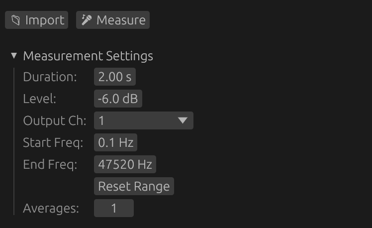
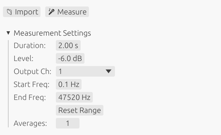
⚠️ Safety Warning
Low frequency content can damage small drivers:
- Sweeps starting below 100 Hz contain high-energy bass content
- Never measure unprotected tweeters or midrange drivers with full-range sweeps
- High excursion at low frequencies can cause mechanical damage or voice coil failure
- For tweeters: Use start frequency >1000 Hz
- For midrange: Use start frequency >200-500 Hz (depending on driver specs)
- Always verify your driver’s rated frequency range before measurement
When measuring individual drivers, adjust the start frequency to match the driver’s safe operating range.
Important note on driver protection methods:
If you use an external high-pass filter (physical or DSP) to protect a driver during measurement instead of adjusting the sweep start frequency, be aware that:
- The filter will affect the phase response and group delay of the measurement
- This phase shift will be captured in the impulse response
- If you later remove or change the protection filter, the driver alignment will be incorrect
- Recommendation: Protect drivers by setting the appropriate sweep start frequency rather than using external filters
- This ensures accurate phase and timing measurements without filter-induced artifacts
Duration
Length of the sweep signal in seconds.
- Range: 1 to 15 seconds
- Shorter (1-3s): Faster measurements, lower frequency resolution, reduced harmonic distortion accuracy
- Longer (5-15s): Better low-frequency resolution, improved SNR, better harmonic distortion measurement
- Recommended: 5-7 seconds for full-range measurements
Benefits of longer sweeps:
- Improved signal-to-noise ratio for harmonic distortion analysis
- More reliable detection and measurement of weak harmonics
- Better frequency resolution in the bass region
⚠️ Important: Longer sweeps deliver more energy to the driver at low frequencies because exponential sweeps spend more time in the bass region. For drivers with limited excursion capability, longer sweeps may require:
- Raising the start frequency to avoid the lowest frequencies
- Reducing the sweep level (amplitude) to limit excursion
- Monitoring the driver during measurement to ensure it doesn’t bottom out
Amplitude
Output level of the sweep signal.
- Range: -50 to 0 dB
- Purpose: Control the acoustic level of the measurement
- Typical: -12 to -6 dB for moderate levels
- Maximum (0.0): Full digital scale output
Adjust amplitude based on driver sensitivity and desired measurement level. Too low may result in poor SNR; too high may cause clipping, distortion or damage.
Start Frequency
Cutoff frequency for the 4th-order Butterworth high-pass filter applied to the sweep for driver protection.
- Default: 1 Hz (captures near-DC response)
- Range: 1 Hz to 20 kHz
- Full-range: 20 Hz (typical for full-bandwidth measurements)
- Subwoofers: 10-20 Hz for low-frequency drivers
- Tweeters: >1000 Hz for high-frequency analysis only (protect from low frequency damage)
- Midrange: >200-500 Hz depending on driver specifications
Understanding the Butterworth Filter Protection
LinFIR applies a 4th-order Butterworth high-pass filter to the sweep signal with cutoff frequency fc = Start Frequency. This provides:
- Attenuation at cutoff: -3 dB at the Start Frequency
- Roll-off below cutoff: -24 dB/octave (deterministic, frequency-independent)
- Minimal pre-ringing: Butterworth maximally-flat passband characteristic
- Continuous protection: Applied across the entire sweep duration
⚠️ Critical positioning guideline:
Because of the -3 dB attenuation at the cutoff frequency, set Start Frequency slightly below your desired passband start, but always above driver safety limits:
- Example: For 80 Hz passband → set Start Frequency to 60-70 Hz
- This accounts for the -3 dB attenuation while ensuring full response in the desired band
- For tweeters: position above resonance frequency (fs) to avoid damage
- For woofers: set at a frequency that limits excursion to safe levels
⚠️ Important: Setting the start frequency too low for small drivers can cause mechanical damage. Always verify your driver’s rated frequency range and adjust accordingly.
For full-range measurements of complete speaker systems, 20 Hz is appropriate. For individual driver measurements, adjust to the driver’s safe operating range.
High Frequency (Automatic)
The high frequency limit is automatically calculated to optimize harmonic distortion measurement quality.
- Calculation: Based on sample rate - set to 1/48 octave before Nyquist frequency
- Range: Typically ~23.5 kHz at 48 kHz sample rate, ~47 kHz at 96 kHz
- Display: The actual calculated frequency is shown in the UI (read-only)
- Optimization: Ensures best separation and detectability of harmonic components (H2-H4)
Why automatic? The high frequency is chosen to provide optimal spacing between the fundamental and its harmonics in the time domain, ensuring accurate distortion measurement. Manual adjustment is not necessary and could compromise measurement quality.
Reset Start Freq Button
Quickly restore the start frequency to its default value:
- Action: Sets Start Freq to default frequency (configured in Audio Settings)
- Use: Return to default start frequency after using restricted frequency ranges for driver protection
Driver Protection and Automatic Windowing
LinFIR applies a sophisticated combination of 4th-order Butterworth high-pass filtering and frequency-domain cosine windowing to protect drivers while ensuring clean measurements.
Butterworth High-Pass Filter for Driver Protection
A 4th-order Butterworth high-pass filter with cutoff frequency fc = Start Frequency is continuously applied across the entire sweep for deterministic driver protection:
Filter Characteristics:
- Cutoff frequency (fc): Set by the Start Frequency parameter
- Attenuation at fc: -3 dB (Butterworth characteristic)
- Roll-off: -24 dB/octave below cutoff (4th order)
- Pre-ringing: Minimal (Butterworth provides best balance)
Why Butterworth?
- Provides deterministic, frequency-independent protection slope
- Minimal pre-ringing compared to steeper filters
- Smooth passband without ripple
- Predictable behavior for all driver types
Protection Mechanism:
- Exponentially reduces energy below the cutoff frequency
- Protects tweeters from low-frequency voltage (thermal damage)
- Limits woofer excursion at sub-bass frequencies (mechanical damage)
- Applied in frequency domain for continuous, artifact-free protection
Understanding the Need for Windowing
When a sweep signal starts or ends abruptly at specific frequencies, it creates discontinuities in the time domain. These discontinuities manifest as Gibbs oscillations in the frequency domain near sharp cutoffs.
These artifacts are not physical - they’re mathematical consequences of abrupt spectral transitions and can mask real acoustic behavior.
How Automatic Windowing Works
LinFIR combines the Butterworth filter with smooth cosine windowing at the boundaries:
Low-Frequency: Butterworth + Cosine Fade-In:
- Butterworth filter (fc = Start Frequency) provides continuous -24 dB/octave protection
- First 1/8 octave uses cosine taper combined with Butterworth to force clean 0 dB at sweep start
- Smooth transition eliminates pre-ringing artifacts
- Combined protection: cosine windowing × Butterworth filtering
High-Frequency Fade-Out:
- Begins at the automatically calculated high frequency (1/48 octave before Nyquist)
- Gradually decreases amplitude using a cosine taper
- Physical sweep extends up to 1/96 octave before Nyquist frequency
- Optimized to maximize harmonic distortion SNR
Adaptive Behavior:
- Fade-out is always applied for optimal high-frequency behavior
- This ensures the sweep always covers its full intended bandwidth with continuous protection
Benefits of Combined Protection
Driver Safety:
- Deterministic -24 dB/octave roll-off below Start Frequency
- Continuous protection without sudden energy changes
- Suitable for all driver types with appropriate frequency selection
Clean Impulse Responses:
- Well-defined peaks without oscillations
- Minimal pre-ringing and post-ringing
- Accurate representation of system behavior
Optimized for Distortion Analysis:
- High frequency chosen to maximize harmonic separation
- Better signal-to-noise ratio for harmonic distorsion detection
No Configuration Required:
- Works optimally for all measurement scenarios
- Eliminates need for user windowing decisions
- Consistent, predictable behavior
Best Practices for Frequency Range Selection
Start Frequency: Driver Protection
The Start Frequency is critical for protecting drivers from damage. Loudspeakers can be damaged by two mechanisms:
1. Over-excursion (mechanical damage)
- Occurs when the cone reaches its physical limits and “bottoms out”
- Results in distortion, mechanical stress, and potential permanent damage
- Most critical for medium to large woofers with high motor force
2. Voice coil overheating (thermal damage)
- Low frequencies behave like DC current, causing excessive heat buildup
- Most critical for midrange drivers and tweeters
- Sending bass frequencies to a tweeter is equivalent to feeding it DC current, which can burn the voice coil
- Small voice coils have limited thermal mass and dissipate heat poorly
Recommended approach by driver type:
Woofers and Subwoofers:
- Adjust Start Frequency to avoid over-excursion
- Use driver simulations to predict excursion limits (e.g., VituixCAD, WinISD)
- Start frequency should be below or at the driver’s resonance frequency for accurate measurement
- Example: 12“ woofer with 15mm Xmax → start at 20-30 Hz to avoid mechanical limits
Tweeters:
- Place Start Frequency well above the driver’s resonance frequency
- Avoid exciting the resonance peak which causes extreme excursion and heat
- Must still measure the useful passband including the crossover region
- Example: Tweeter with 800 Hz resonance and 2 kHz crossover → start at 1000-1500 Hz
- This captures the crossover transition while protecting against resonance excitation
Midrange drivers:
- Balance between capturing low-frequency rolloff and avoiding resonance excitation or over-excursion
- Typically start 100-300 Hz below the intended crossover frequency
- Monitor excursion if measuring near resonance frequency
- Example: Midrange crossing at 500 Hz with 200 Hz resonance → start at 300-400 Hz
General rule:
- Always verify your driver’s specifications before measurement
- When in doubt, start conservative (higher frequency) and lower gradually while monitoring
Starting a Measurement
Measure Button (🎤 Measure)
Clicking the 🎤 Measure button initiates the sweep measurement process.
Default behavior (confirmation enabled):
- Click 🎤 Measure
- Confirmation dialog appears with warnings:
- Check microphone and speaker positioning
- Set appropriate gain levels to avoid clipping
- The sweep will be audible
- Windows-specific timing warning (if applicable)
- Click Start Measurement to proceed or Cancel to abort
- Sweep plays and records automatically
- IR is processed and validated
Direct mode (confirmation disabled):
- Measurement starts immediately when clicking 🎤 Measure
- No confirmation dialog shown
- Useful for quick repeated measurements
Disabling Confirmation Dialog
To disable the confirmation dialog:
- Open Settings (Cmd/Ctrl + ,)
- Navigate to Audio Settings
- Enable “Skip confirmation dialog” option
- Measurements will now start immediately
Warning: Disabling confirmation means sweeps start instantly. Ensure your setup is ready before clicking the button to avoid unexpected loud sweeps.
Stopping a Measurement
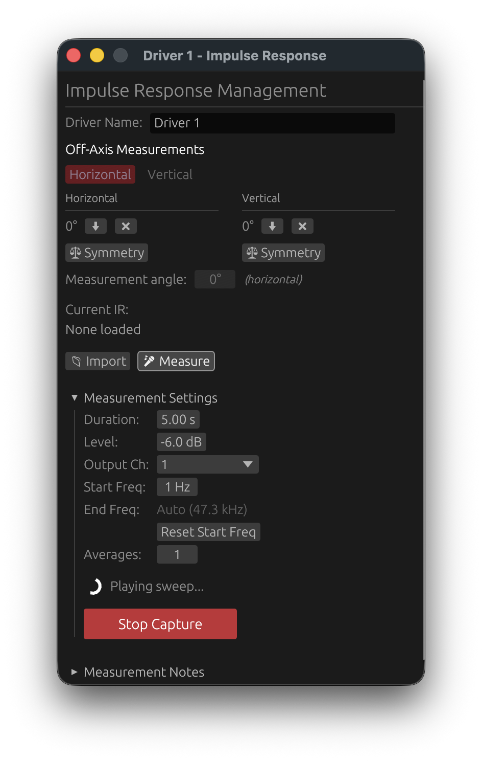
Emergency Stop
You can interrupt a sweep at any time during capture:
- Stop Capture button: Click the red button that appears during measurement
- Spacebar: Press the spacebar key for instant interruption
When to use emergency stop:
- Incorrect parameters: Realized the frequency range or level is inappropriate for the driver
- Excessive gain: Input signal is clipping or distorting
- Driver protection: Driver showing signs of stress (unusual sounds, excessive excursion)
- Environmental issues: Unexpected noise or interference occurred
The measurement will stop immediately when interrupted. You can then adjust parameters and start a new measurement.
Automatic Stop on Clipping
LinFIR monitors the input signal in real time during the entire sweep and will automatically cancel the measurement the moment clipping is detected — without waiting for the sweep to finish.
What happens:
- The input callback continuously tracks the peak level of every audio buffer
- As soon as any sample reaches digital full-scale (±1.0), the sweep is immediately faded out and stopped
- A notification toast identifies the cancellation as clipping-triggered
Toast messages:
- “Measurement cancelled: clipping detected! Reduce the output level or input gain and try again.” — clipping occurred on the main measurement channel
- “Measurement cancelled: clipping on the timing reference channel! Reduce the timing reference output level.” — clipping occurred on the timing reference channel (Electric or Acoustic mode); detected in the first ~1.2 s of the sweep, before the main sweep begins
Why this matters:
- Without real-time detection, clipping is only discovered at the end of the sweep after wasting the full measurement duration
- Immediate stop prevents unnecessary acoustic exposure of the driver to a potentially damaging clipped signal
- The automatic stop uses the same graceful fade-out as the manual Stop Capture button — no abrupt clicks
What to do:
- Reduce the audio interface input gain
- Lower the sweep amplitude
- Move the microphone farther from the driver
- For timing reference clipping: lower the timing reference output level in Audio Settings
Automatic Early Stop on Weak Timing Reference Signal
When a timing reference is active (Electric or Acoustic mode), LinFIR checks the level recorded on the timing reference channel shortly after the chirp ends, and cancels automatically if the signal was too weak to be reliable.
What happens:
- During the chirp window, the peak level on the timing reference input channel is continuously tracked
- After the end of the chirp, the accumulated peak is evaluated
- If the peak never exceeded −25 dBFS, the measurement is cancelled immediately (before the main sweep even begins)
- Toast message: “Measurement cancelled: timing reference signal too low (X.X dBFS < −25 dBFS). Check the timing reference channel connection and level.”
Why this matters:
- A weak timing reference signal makes latency detection unreliable or impossible
- Catching the problem immediately — before the full sweep — avoids wasting the measurement time
What to do:
- Check that the timing reference channel is connected correctly
- Increase the timing reference output level in Audio Settings
- For Acoustic mode, verify that the microphone can capture the high-frequency chirp (5–20 kHz)
Automatic Early Stop on Low Signal (Multi-Average)
When a measurement is configured with 2 or more averages, LinFIR checks the signal level at the end of the first sweep — before the second sweep begins — and cancels automatically if the signal was too weak.
What happens:
- During the first sweep, the peak input level is continuously tracked
- ~200 ms into the post-sweep silence (after the sweep signal has ended), the accumulated peak is evaluated
- If the peak never exceeded −25 dBFS, the measurement is cancelled before the second average starts
- Toast message: “Measurement cancelled: signal too low on first sweep (< −25 dBFS). Increase input gain or move the microphone closer.”
Why this matters:
- A low-level signal produces a poor signal-to-noise ratio; averaging more sweeps will not fix it
- Stopping after the first sweep avoids wasting time on subsequent averages that would yield unusable results
What to do:
- Increase the audio interface input gain
- Move the microphone closer to the driver
- Increase the sweep amplitude (Output Level in Sweep Parameters)
Note: The multi-average level check requires ≥ 2 averages. For single-sweep measurements, the level check occurs after the full capture completes and the result is simply rejected if too low. The timing reference level check (above) applies regardless of the number of averages.
Window Behavior During Capture
To ensure reliable interruption, the IR Management window:
- Remains on top of all other windows during measurement
- Maintains keyboard focus throughout the capture
- Returns to normal window behavior when measurement completes or is stopped
This prevents accidental loss of control during the sweep. The spacebar shortcut will always work, even if you accidentally click elsewhere during measurement.
Level Recommendations
Target levels for best measurement quality:
- Optimal: -6 dB to -12 dB
- Acceptable: -12 dB to -20 dB
- Too low: Below -25 dB (poor SNR, noisy measurements)
- Too high: Above -3 dB (risk of clipping)
Quality Validation
LinFIR automatically validates each capture and rejects poor-quality measurements.
Clipping Detection
- Criteria: Any sample reaching digital full-scale (±1.0)
- Result: Capture rejected immediately
- Reason: Clipping introduces harmonic distortion that corrupts the impulse response
Solution: Reduce input gain or lower acoustic level (move microphone farther or reduce driver volume).
Level Check
- Criteria: Peak level must be ≥ -25 dB
- Result: Capture rejected if too low
- Reason: Low levels result in poor signal-to-noise ratio
Solution: Increase input gain, raise driver volume, or move microphone closer.
Best Practices
Microphone Positioning
- On-axis measurements: Position microphone directly in front of driver at typical listening distance
- Listening position: For room measurements, place microphone at primary listening position
- Height: Maintain consistent height, typically at seated ear level (90-150 cm)
- Distance:
- Farfield recommended: 0.5-1.5 meters with windowing (quasi-anechoic technique)
- Avoid nearfield: Nearfield measurements (<20cm) capture reactive near-field effects (evanescent waves) that don’t propagate to listening position
- Consistency critical: Use the same microphone position for all drivers to maintain correct relative phase and amplitude relationships
Why Avoid Nearfield for Multi-Way Systems?
Physical limitations:
- At different distances, the reactive impedance field varies between drivers
- Nearfield captures evanescent waves (reactive air-driver coupling) that decay exponentially and never reach the listener
- These reactive effects create phase rotations and magnitude errors that don’t represent real acoustic radiation
Practical consequences:
- Impossible to maintain consistent distance across drivers of different sizes (tweeter vs woofer require different nearfield distances)
- Phase relationships corrupted: Crossover alignment becomes unreliable when drivers measured at different distances
- Baffle effects missed: Nearfield ignores diffraction and baffle step that dominate the actual system response
Recommended approach:
- Measure at 0.5-1m distance (same position for all drivers)
- Use time windowing to eliminate room reflections (quasi-anechoic)
- Captures correct far-field radiation including baffle interactions
- Maintains phase coherence between drivers for accurate crossover design
Acoustic Environment
- Minimize noise: Turn off HVAC, fans and noisy appliances during measurement
- Reduce reflections: For anechoic-like measurements, gate reflections using time windowing
- Room measurements: Accept reflections, use time windowing to exclude late reflections only
- Outdoor measurements: Recommended to avoid room gain and obtain better results at low frequencies
Measurement Microphone
- Type: Use calibrated measurement microphone (e.g., UMIK-1, Earthworks M23, Beyerdynamic MM-1)
- Calibration: Load manufacturer calibration file before measurements
- Quality: Consumer microphones lack flat frequency response and will give inaccurate results
Gain Staging
- Start with moderate input gain
- Run a test sweep
- Check peak level indicator
- Adjust gain to achieve -6 dB to -12 dB peaks
- Re-measure if clipping or too low
Sweep Duration
- Full-range (20 Hz - 20 kHz): 5-7 seconds recommended
- Limited bandwidth: Shorter sweeps acceptable (2-3 seconds)
- Very low frequencies (< 20 Hz): Use longer sweeps (7-10 seconds)
Capture Rejection Messages
“Capture Rejected - Clipping Detected”
Cause: Input signal exceeded digital full-scale.
Solutions:
- Reduce audio interface input gain
- Lower driver volume
- Move microphone farther from driver
- Check gain staging in signal chain
“Capture Rejected - Signal Too Low”
Cause: Peak level below -25 dB threshold.
Solutions:
- Increase audio interface input gain
- Raise driver volume
- Move microphone closer to driver
- Verify microphone connection and phantom power
- Check audio routing and device selection
Advanced Topics
Sweep Output Channel
In the IR Management window, you can select which output channel plays the sweep:
- Purpose: Direct sweep to specific amplifier channel
- Room Calibration: Select channel connected to main loudspeaker (excluding timing reference)
- Multi-way systems: Measure each driver individually by routing to appropriate channel
Multiple Measurements
For averaging or multi-position captures in Room Calibration mode:
- Configure timing reference (Electric or Acoustic) in Audio Settings
- Capture first measurement (this becomes the timing reference)
- Capture subsequent measurements at different positions or conditions
- In Room Calibration mode, measurements are automatically aligned using GCC-PHAT
Measurement Averaging
Averaging works on all platforms without requiring a timing reference:
- LinFIR uses a continuous capture approach: one recording containing N consecutive sweep segments
- After alignment, segments are extracted and averaged to reduce noise
- Operating system scheduler jitter only affects the initial timing, not the relative timing between segments
Timing reference recommendation:
- Not required for averaging (continuous capture eliminates timing inconsistency between segments)
- Still recommended on Windows for absolute timing accuracy if comparing measurements across drivers
- Mac OS: System clock is already reliable for all timing needs
Auto-Scan with a Rotation Table 🔒
Requires: a valid LinFIR license and a connected rotation table (Pololu Tic or GRBL/Arduino — see Rotation Table).
The auto-scan feature drives the rotation table through a configurable angle range and measures an impulse response at each step — fully automatically.
Starting Auto-Scan
In the IR Management window, when a rotation table is connected and a license is active, a ▶ Scan button appears alongside the standard 📁 Import and 🎤 Measure buttons.
Before clicking ▶ Scan, configure:
- Axis selector (Horizontal / Vertical) — determines whether measurements are stored as horizontal or vertical off-axis
- Auto-scan range — min angle, max angle (e.g. −90° to +90°)
- Step — angular increment between measurements (e.g. 10°)
| Parameter | Default | Description |
|---|---|---|
| Min angle | −90° | First off-axis angle (negative side) |
| Max angle | +90° | Last off-axis angle (positive side) |
| Step | 10° | Angular increment between captures |
What Happens
- LinFIR builds a queue of angles:
0°, +step, +2×step, …, max, −step, −2×step, …, min - Already-measured angles are skipped automatically
- For each remaining angle:
- The table moves to the target angle
- LinFIR waits 500 ms for the table to settle after it stops moving
- A sweep capture starts (with your current sweep parameters)
- When the capture completes, the next angle is queued
- A “Auto-scan complete” toast is shown when all angles are done
State Machine
stateDiagram-v2
    [*] --> Moving : ▶ Scan clicked
    Moving --> Settling : table stopped at target
    Moving --> [*] : timeout (30 s)
    Settling --> Capturing : 500 ms elapsed
    Capturing --> Moving : capture done, angles remain
    Capturing --> [*] : all angles done
Progress Display
While auto-scan is running, a spinner and status line appears below the buttons:
⟳  Moving to 30°… (7 remaining)
⟳  Settling at 30°… (7 remaining)
⟳  Measuring 30°… (7 remaining)
Stopping Auto-Scan
- Click the ■ Stop button (replaces ▶ Scan while active)
- Press Space (also stops any capture in progress)
Both methods immediately halt the current capture and cancel the remaining queue.
Timeout
If the table takes more than 30 seconds to reach a target angle, auto-scan is cancelled with an error toast. Check mechanical issues or increase the move speed on your controller.
For hardware setup, controller configuration, and troubleshooting, see Rotation Table.
Technical Details
Exponential Sine Sweep (Farina Method)
LinFIR uses an exponential sine sweep (ESS) for impulse response measurements, based on Angelo Farina’s method:
Basic ESS Properties:
- Frequency distribution: Equal energy per octave
- Low-frequency emphasis: More time spent at low frequencies
- Deconvolution: Analytical inverse filter applied to extract impulse response
Harmonic Distortion Detection:
The exponential sweep provides natural time separation of harmonic distortion products:
- Deterministic harmonic positions: All harmonic distortion products (H2, H3, H4) appear at predictable time positions in the deconvolved impulse response
- Time separation formula: Δt(Hₙ) = (T/ln(f₂/f₁)) × ln(n)
- H2 (2nd harmonic) appears at: Δt × ln(2) ≈ 0.693 Δt before the main peak
- H3 (3rd harmonic) appears at: Δt × ln(3) ≈ 1.099 Δt before the main peak
- H4 (4th harmonic) appears at: Δt × ln(4) ≈ 1.386 Δt before the main peak
Deconvolution
After recording the sweep response LinFIR automatically:
- Compute the inverse sweep signal
- Convolve recorded response with inverse sweep
- Extract impulse response from convolution result
- Apply microphone calibration (if loaded)
- Validate quality (clipping and level check)
Quality Criteria
- Clipping: Zero tolerance - any sample at ±1.0 rejects capture
- Minimum level: -25 dB peak threshold ensures adequate SNR
- These are conservative: Ensure high-quality measurements
Workflow Example
- Configure Audio: Set input/output devices, sample rate, buffer size
- Load Calibration: Import microphone calibration file (if available)
- Position Microphone: Place at measurement location
- Set Sweep Parameters: Duration = 5s, Amplitude = -6 dB, Full range (20 Hz - 22 kHz)
- Test Sweep: Run a test to check levels
- Adjust Gain: Aim for -6 dB to -12 dB peak levels
- Measure: Click 🎤 Measure button to record impulse response
- Confirm: Click Start Measurement in the confirmation dialog (or skip if disabled in settings)
- Verify: Check impulse response graph for quality
- Repeat: Capture additional measurements as needed
Driver Processing
Each driver in LinFIR can be individually processed with a comprehensive signal chain combining FIR crossovers, FIR correction filters, IIR equalization, polarity inversion, and time/gain adjustments.
The processing chain for each driver follows this order:
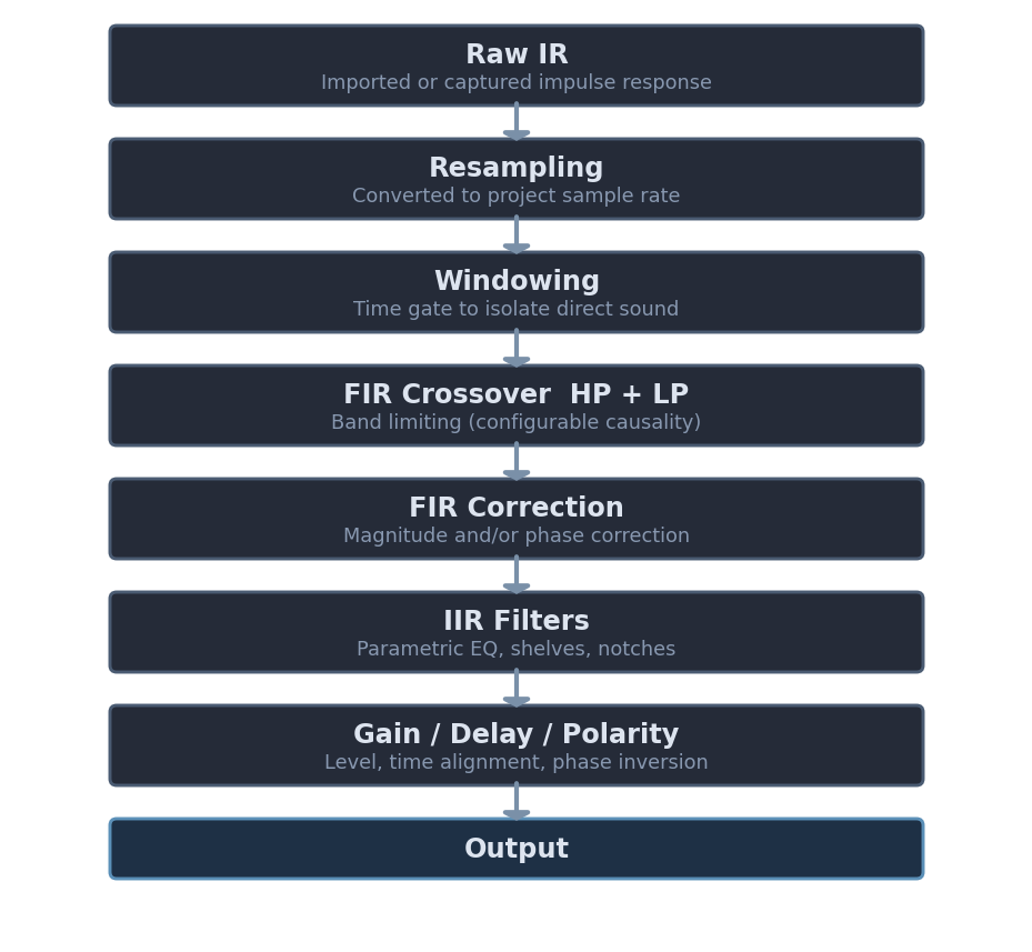
Driver Management
Adding and Removing Drivers
Add Driver:
- Maximum: 10 drivers per project
- Click ➕ Add Driver button in the Drivers toolbar
- New driver initialized with default settings
Remove Driver:
- Click 🗑 button in the driver’s bottom action bar
- Only visible when more than one driver is present
- Hidden in Hypex mode (driver count is locked by the selected model)
Copy / Paste Driver Parameters:


- Click 📋 to copy all parameters of a driver to the clipboard
- IRs and driver name are not copied — only filter and DSP settings
- Copied parameters include: FIR/IIR filters, gain, time delay, polarity, tap lengths, windowing, correction settings, mic calibration, and sweep parameters
- Click 📥 to paste the clipboard parameters onto another driver
- The target driver’s IRs and name are preserved
- The 📥 button is grayed out when no parameters have been copied yet
- Useful for duplicating crossover or EQ settings across multiple drivers without redoing each one manually
Driver Organization:
- Drivers are organized in collapsible sections in the left toolbar
- Each section shows the driver name (or “Driver 1”, “Driver 2”, etc. if unnamed)
- Driver names are automatically set when importing impulse responses
Driver Controls
Enable/Disable and Solo
Enable Toggle:
- Button to enable/disable individual drivers
- Disabled drivers are excluded from calculations and the summed response
- Useful for A/B testing or isolating specific drivers
Solo Button:
- Instantly disables all other drivers and enables only the selected driver
- Quick way to review individual drivers in isolation
All Button:
- Re-enables all drivers simultaneously
- Convenient after using Solo mode
Driver Interface Overview
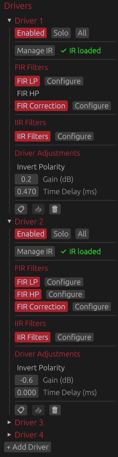
Each driver’s interface provides access to all processing and configuration options, organized into three main sections:
- Manage IR: Import/capture impulse responses and configure windowing
- FIR Filters: Low-pass, high-pass, correction filters, and FIR offset delay (if enabled in global settings)
- IIR Filters: Parametric EQ and filter design
- Driver Adjustments: Polarity inversion, gain, and time delay adjustments
The following sections detail each of these components.
Impulse Response Management
Loading Impulse Responses
Click Manage IR to open the impulse response management window for:
- Importing pre-recorded impulse responses
- Capturing new measurements via audio interface
- Configuring IR windowing parameters
- Managing off-axis measurements for directivity analysis
See IR Management for detailed documentation.
IR Status Indicator:
- Gray “No IR loaded”: Driver has no impulse response
- Green “✅ IR loaded”: Valid impulse response loaded
⚠️ Note: A loaded impulse response is required for filter design and correction. Without an IR, only theoretical filter responses can be displayed.
Target DSP Settings
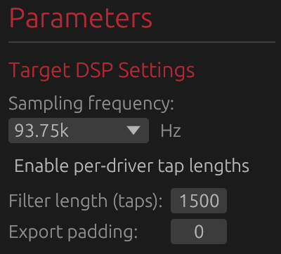
The Target DSP Settings section configures fundamental parameters that determine filter design constraints and export characteristics. These settings directly impact frequency resolution, latency, and compatibility with your target DSP platform.
⚠️ Note: You can change these settings at any time to match different DSP characteristics, but doing so will affect the precision, effectiveness, delays, and slopes of any FIR filters you have already set.
Sample Rate
Options: 44.1 kHz, 48 kHz, 88.2 kHz, 93.75 kHz, 96 kHz, 176.4 kHz, 192 kHz
Current project: Fixed at project creation
The sample rate is set when creating a new project and cannot be changed afterward. It determines:
- Nyquist frequency: Maximum representable frequency (sample rate / 2)
- Filter frequency resolution: Higher rates provide finer resolution
- Latency: For a given tap count, higher sample rates have lower latency in milliseconds
- DSP compatibility: Must match your target DSP platform’s operating sample rate
Common choices:
- 44.1 kHz: Compact DSP platforms with limited processing power
- 48 kHz: Professional audio standard, most DSP platforms
- 88.2 kHz: High-resolution audio (2× CD rate, relatively uncommon for DSP)
- 93.75 kHz: Hypex DSP platforms (FA123, FA253, FA502, etc.)
- 96 kHz: High-resolution audio, some professional DSP platforms
- 176.4/192 kHz: Ultra-high resolution - only when DSP platform specifically requires it
Enable per-driver tap lengths
Default: Disabled (shared tap length applies to all drivers)
When disabled (default):
- Single Filter length (taps) control in Target DSP Settings applies to all drivers
- Single Export padding control in Target DSP Settings applies to all drivers
- Simpler configuration for uniform systems
- All drivers use the same FIR filter length
When enabled:
- Filter length (taps) and Export padding controls move from Target DSP Settings to individual driver sections
- Each driver gets its own controls in its collapsible section
- Allows optimization: fewer taps for tweeters, more for woofers/subwoofers
- Useful for minimizing DSP load while maintaining quality where needed
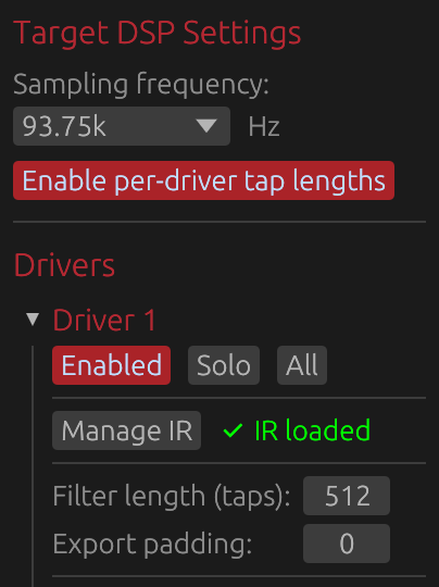
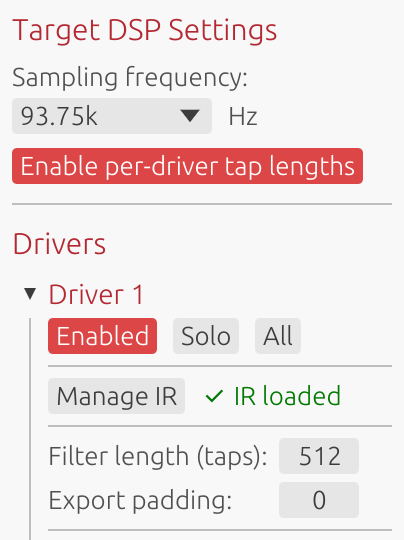
Example use case: Use 2048 taps for subwoofer (needs low-frequency resolution), 512 taps for tweeter (high frequencies need less resolution).
⚠️ Note: Linear phase FIR filters and phase-correction FIR filters introduce noticeable delays that depend on the number of taps. Different tap lengths between drivers will likely introduce time misalignments, which you can correct using the Time Delay parameter in the Driver Adjustements section.
Filter Length (Taps)
Range: 32 to 65536 taps
Default: 512 taps
Location:
- Shared mode (per-driver tap lengths disabled): In Target DSP Settings section - applies to all drivers
- Per-driver mode (per-driver tap lengths enabled): In each driver’s collapsible section
Controls the length of all FIR filters for this driver (crossover and correction filters).
Frequency Resolution:
- Resolution (Hz) = Sample Rate / Tap Count
- Example at 48 kHz: 512 taps = 93.75 Hz resolution, 4096 taps = 11.72 Hz resolution
- Lower frequencies need more taps for precise control
Latency (Linear-Phase):
- Latency = (Taps / 2) / Sample Rate
- Example at 48 kHz: 512 taps = 5.33 ms, 4096 taps = 42.67 ms
- Can be reduced using Causality control at the cost of phase linearity
Practical guidelines:
- 256-512 taps: Tweeters, minimal latency applications
- 512-2048 taps: Most crossover and correction applications
- 2048-4096 taps: Typical maximum for full-range loudspeaker designs
- 4096-8192 taps: Subwoofer correction, room correction
- 8192-16384 taps: Specialized low-frequency correction below 20 Hz
- >16384 taps: Rarely needed (extreme cases, research purposes)
Trade-offs:
- ✅ More taps = better frequency resolution, steeper filter slopes, more precise correction
- ❌ More taps = higher latency (for linear-phase), increased DSP load, larger export files
Export Padding
Range: 0 to 65536 taps
Default: 0
Location:
- Shared mode (per-driver tap lengths disabled): In Target DSP Settings section - applies to all drivers
- Per-driver mode (per-driver tap lengths enabled): In each driver’s collapsible section
Adds zero-padding only to exported files, without affecting internal processing or design.
Purpose:
- Some DSP platforms require specific filter lengths (e.g., powers of 2: 512, 1024, 2048, 4096)
- Padding allows meeting DSP requirements without changing internal design
- Does not affect latency, delay, or any graph displays
How it works:
- Internal design: Uses configured tap count
- Export: Appends zeros to reach (Taps + Padding) length
- Frequency response remains identical (zero-padding doesn’t alter frequency content)
Example scenario:
- Design with 3000 taps, DSP requires power-of-2 → Set padding to 1096 → Exports 4096 taps
When not needed: If your DSP accepts arbitrary filter lengths, leave padding at 0.
FIR Crossover Filters
FIR Low-Pass Filter
Enable: Toggle FIR LP button
Configure: Click Configure button (only available when enabled)
Applies a linear-phase low-pass filter to limit the driver’s high-frequency response.
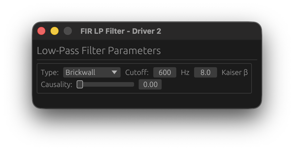
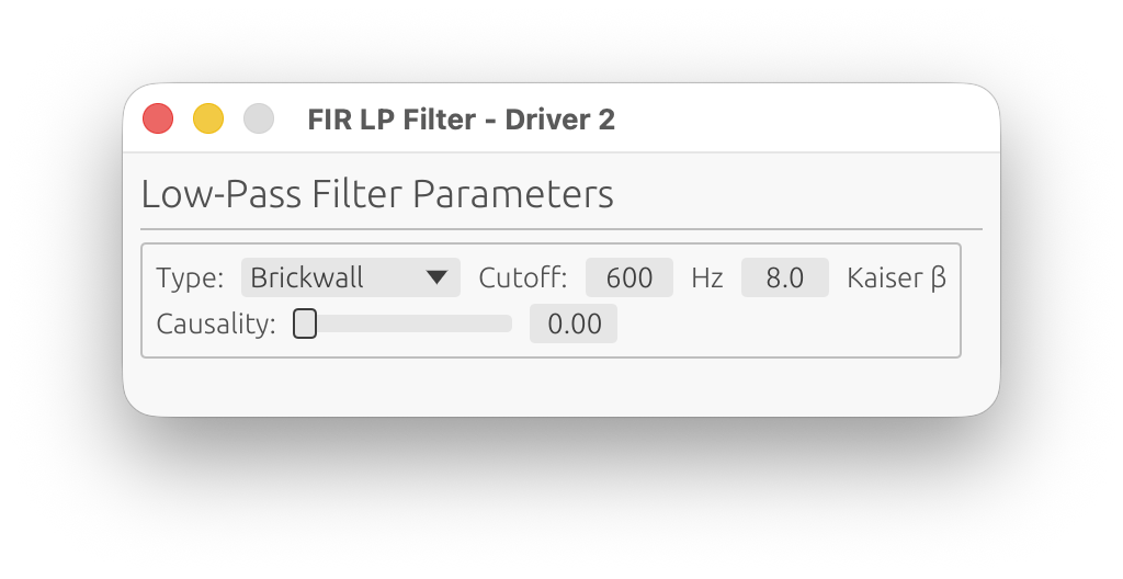
Parameters:
Filter Type
Choose the crossover filter design:
-
Brickwall: Ideal brickwall (Sinc) filter using Kaiser window
- Sharpest possible slope
- Controlled transition width via Kaiser β parameter
-
Linkwitz-Riley: Linkwitz-Riley aligned response
- -6 dB at crossover frequency (sums to 0 dB when paired with matching HP)
- Constant power summing when combined with complementary HP filter
- Order: 2, 4, 6, 8, or 10 (even orders only)
-
Butterworth: Classic analog-style Butterworth response
- Maximally flat magnitude in passband
- Order: 1 to 10
-
Bessel: Bessel/Thomson response
- Originally optimized for linear phase response and minimal group delay variation
- Gentler roll-off than Butterworth
- Order: 1 to 10
Cutoff Frequency
Range: 1 Hz to Nyquist frequency
Step: 1 Hz
The -6 dB point for brickwall filters, or the characteristic frequency for Butterworth/Linkwitz-Riley filters.
Typical values:
- Woofer-Midrange: 300-800 Hz
- Midrange-Tweeter: 2-4 kHz
Kaiser β
Range: 0.0 to 50.0
Default: 8.0
Controls the Kaiser window applied to the FIR filter impulse response. This parameter adjusts the trade-off between transition width and stopband ripple:
For Brickwall filters:
- Lower values (3-5): Narrower transition BUT higher stopband ripple (higher sidelobe levels)
- Moderate values (6-10): Balanced transition width and stopband attenuation
- Higher values (12-20): Wider transition BUT lower stopband ripple (better attenuation)
For Butterworth, Linkwitz-Riley and Bessel filters:
- Controls FIR windowing to suppress ringing and ripple in the stopband
- Lower values (3-5): Sharper response BUT higher ripple/ringing in stopband
- Moderate values (6-10): Good balance between sharpness and ripple suppression
- Higher values (12-20): Gentler response BUT maximum ripple suppression
Common choices:
- β = 5: Narrow transition with noticeable ripple (not necesarrily audible as the complementary driver will mask it)
- β = 8-9: Standard crossover design, good compromise
- β = 12-15: Wide transition with excellent stopband attenuation
Order (Butterworth/Linkwitz-Riley/Bessel only)
Butterworth/Bessel Range: 1, 2, 3, 4, 5, 6, 7, 8, 9, 10
Linkwitz-Riley Range: 2, 4, 6, 8, 10 (even only)
Higher order = steeper slope (more dB/octave attenuation).
- 2nd order: 12 dB/octave (gentle slope)
- 4th order: 24 dB/octave (most common for LR designs)
- 6th order: 36 dB/octave
- 8th order: 48 dB/octave (steep slope)
Causality
Range: 0.0 (linear-phase) to 1.0 (minimum-phase)
Default: 0.0 (linear-phase)
Interpolates between linear-phase and minimum-phase behavior for the FIR crossover filter.
Purpose: Limits the delay introduced by the FIR filter while maintaining steeper slopes than IIR filters, at the cost of phase distortion.
Linear-Phase (0.0):
- Symmetric pre- and post-ringing
- Constant group delay across all frequencies
- No phase distortion
- Highest latency (taps/2 samples)
- Best for high-fidelity applications
Minimum-Phase (1.0):
- No pre-ringing (all energy is causal)
- Variable group delay
- Phase follows magnitude via Hilbert transform
- Minimal latency
- Best for low-latency applications
Intermediate values:
- Blend between linear and minimum phase
- Reduced pre-ringing compared to linear-phase
- Some phase distortion compared to linear-phase
- Lower latency than full linear-phase
Typical values:
- 0.0: High-fidelity systems, studio monitors, reference designs
- 0.5: Balanced compromise
- 1.0: Low-latency systems, live sound, PA applications
Trade-off: Increasing causality reduces latency but introduces phase distortion. For multi-driver systems, matching causality settings across all drivers maintains phase coherence.
FIR High-Pass Filter
Enable: Toggle FIR HP checkbox
Configure: Click Configure button (only available when enabled)
Applies a linear-phase high-pass filter to limit the driver’s low-frequency response.
Parameters: Identical to FIR Low-Pass (Type, Cutoff, Kaiser β, Order, Causality)
Linkwitz-Riley and Brickwall Crossover Design: When using complementary LR filters (e.g., woofer LP at 500 Hz + midrange HP at 500 Hz, both 4th order), the combined magnitude response is flat at the crossover point.
FIR Correction Filter
Enable: Toggle FIR Corr button
Configure: Click Configure button (only available when enabled)
Applies frequency-domain magnitude and/or phase correction using the loaded impulse response.
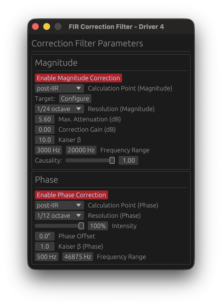
The correction filter window has two main sections: Magnitude and Phase.
Magnitude Correction
Enable Magnitude Correction
Toggle to enable/disable magnitude response correction independently from phase.
Calculation Point
Choose where correction is calculated in the processing chain:
-
pre-IIR: Correction computed from raw IR before IIR filters
- Use when IIR filters are for fine-tuning only
- Simpler, doesn’t account for IIR response
-
post-IIR: Correction computed after IIR filter application
- Accounts for IIR filter effects in the correction calculation
- Use when IIR filters significantly alter the response
- More accurate for complex filter chains
Target Curve
Click Configure to open the target curve configuration window.
Purpose: Define the desired magnitude response for this driver.
See Target Curves for detailed configuration.
Frequency Range
Start Frequency:
- Range: 1 Hz to Nyquist
- Default: 20 Hz
- Lower limit for magnitude correction
End Frequency:
- Range: 1 Hz to Nyquist
- Default: Nyquist
- Upper limit for magnitude correction
Purpose: Restrict correction to a specific frequency range, avoiding correction where measurements are unreliable or correction is undesirable.
Important: Magnitude correction applies a smooth taper (transition zone) at the frequency range boundaries to prevent discontinuities:
- Taper width: Quarter-octave (1/4 octave) above and below the correction range
- Taper function: Raised cosine (smooth fade-in/fade-out)
- Below Start Frequency: Correction weight fades from 0% at
Start / 2^(1/4)to 100% atStart - Above End Frequency: Correction weight fades from 100% at
Endto 0% atEnd × 2^(1/4) - Example: For Start = 200 Hz, the taper begins at 168 Hz. For End = 10 kHz, the taper extends to 11.9 kHz
- Purpose: Ensures smooth transitions without abrupt magnitude steps or phase artifacts
Critical Understanding: Correction Source Signal
The magnitude correction filter is computed from the driver’s impulse response without FIR low-pass or high-pass filters applied (those are applied later in the signal chain). The correction sees:
- ✅ IIR filters (if “post-IIR” calculation mode is enabled)
- ❌ FIR LP/HP crossovers (not applied yet)
Practical Implications:
1. With IIR Crossovers (post-IIR mode):
- The correction attempts to flatten the IIR crossover rolloff
- ⚠️ This removes your crossover slope, which is usually undesirable
- Solution: Limit the frequency range to roughly your driver’s final passband
- Example: For a tweeter with IIR HP at 2 kHz, set correction range to 2.5 kHz - 20 kHz
2. With pre-IIR mode or FIR crossovers:
- The correction sees the driver’s raw natural rolloff
- Risk: Amplifying rolloff increases noise and distortion outside the intended band
- Sometimes helpful: Can improve summation in the crossover transition region
- Solution: Set frequency range to where summation matters, don’t extend further
- Example: For a midrange crossing at 500 Hz and 3 kHz, limit to 400 Hz - 4 kHz
Best Practice: Configure the frequency range to match your driver’s intended operating band considering your crossover strategy, not just where the measurement looks good.
Resolution
Options: 1/48 oct, 1/24 oct, 1/12 oct, 1/6 oct, 1/3 oct
Default: 1/12 octave
Fractional-octave smoothing applied to the measured response before computing the correction filter. This determines the resolution of features that will be corrected.
Purpose: Avoid correcting measurement artifacts (reflections, diffraction ripples, noise) that are not inherent to the speaker’s response.
- 1/48 oct to 1/24 oct: Minimal smoothing - risks correcting artifacts and creating excessive filter complexity
- 1/12 oct: Recommended balance - corrects real speaker behavior while ignoring fine ripples
- 1/6 to 1/3 oct: Heavy smoothing - corrects only broad trends
Key principle: The correction filter resolution should match the reliability of your measurement, not its raw resolution. Narrow features (<1/12 oct) are often artifacts, not real acoustic properties worth correcting.
Recommendation: Use 1/12 octave for typical speaker correction, 1/6 octave for room measurements or when measurement quality is uncertain.
Max. Attenuation (dB)
Range: 0 to 30 dB
Default: 10 dB
Maximum attenuation applied by the magnitude correction filter.
How it works: The correction filter works by “cutting from the top” - it attenuates peaks in the measured response to bring them down toward the target curve. This parameter limits how much attenuation is applied.
Purpose:
- Prevents excessive notching of narrow peaks (which may be measurement artifacts)
- Keeps the correction filter smooth and stable
- Avoids creating deep notches that could be audible as resonances
Typical values:
- 5-8 dB: Conservative correction for well-behaved drivers
- 10 dB: Standard value for most applications
- 12-15 dB: More aggressive correction (check impulse response for artifacts)
- >15 dB: Rarely needed, may indicate measurement issues
Important: The correction filter primarily attenuates rather than boosts. Use Correction Gain (below) to compensate for the overall level reduction.
Correction Gain (dB)
Range: -20 to +20 dB
Default: 4 dB
Gain applied within the correction frequency range to compensate for the attenuation introduced by the magnitude correction filter.
Purpose:
- Restores overall level after attenuation-based correction
- Allows fine-tuning the driver’s output level
- Maintains consistent loudness across the corrected frequency band
Typical values:
- 0-4 dB: Minimal compensation (gentle correction)
- 4-6 dB: Standard compensation for moderate correction
- 6-10 dB: High compensation (use with caution)
⚠️ Warning: Excessive correction gain can cause clipping in the internal DSP signal chain or damage your drivers. Keep gain reasonable (< 6 dB recommended) to maintain headroom. If LinFIR’s clipping detection is enabled (see Settings), you’ll receive warnings about potential clipping.
Kaiser β (Magnitude)
Range: 0.0 to 50.0
Default: 8.0
Kaiser windowing parameter for the magnitude correction FIR filter.
Effect:
- Lower values (3-5): Sharper correction BUT may amplify ripple from crossover filters (LP/HP) if active
- Moderate values (6-10): Good balance between precision and ripple suppression
- Higher values (12-20): Smoother correction, reduced ripple amplification, but less precise
When to adjust:
- If you see excessive ripple in the stopband after applying correction with active crossover filters, increase Kaiser β
- If correction seems too gentle or imprecise, decrease Kaiser β
Recommendation: Start with default 8.0, increase to 12-15 if ripple is problematic with crossover filters active.
Causality (Magnitude)
Range: 0.0 (linear-phase) to 1.0 (minimum-phase)
Default: 1.0 (minimum-phase)
Controls the phase characteristic of the magnitude correction filter.
- 0.0 (Linear-phase): Symmetric pre- and post-ringing, constant group delay
- 1.0 (Minimum-phase): No pre-ringing, all energy is causal, variable group delay
Typical choice: 1.0 (minimum-phase) to avoid pre-ringing artifacts.
Why minimum-phase is preferred: Most acoustic and electronic systems are minimum-phase (magnitude and phase are coupled via Kramers-Kronig relations). Correcting magnitude with a minimum-phase filter automatically corrects the associated phase deviation, providing physically accurate correction. Use 0.0 (linear-phase) only if you specifically need constant group delay with a non-flat target curve and can tolerate pre-ringing.
Phase Correction
Enable Phase Correction
Toggle to enable/disable phase response correction independently from magnitude.
🚫 Non-anechoic measurements: phase correction is strongly discouraged
Phase correction requires clean, accurate phase data. In-room measurements contain reflections, room modes, and position-dependent artifacts that pollute the phase response. Applying phase correction to such data produces unpredictable — and often worse — results.
Only use phase correction with anechoic or near-anechoic measurements (e.g., measurements gated to remove reflections, or made in an anechoic chamber). For in-room measurements, restrict correction to magnitude only.
⚠️ Critical Limitation: Phase Correction vs. Low Latency
You cannot have both near-zero latency FIR filters AND active phase correction. This is a fundamental limitation, not a software bug.
Why this incompatibility exists:
Even if you configure your FIR crossover filters (HP/LP) and FIR magnitude correction with causality = 1.0 (minimum-phase, low latency), which positions the FIR impulse peak near t=0 (left-aligned), enabling phase correction will shift the combined FIR impulse peak to the center (around ntaps/2), introducing significant latency.
The reason is fundamental:
- Phase correction = temporal correction: Phase distortion is fundamentally a time-domain problem (different frequencies arriving at different times)
- To correct temporal defects, you need time: The filter needs temporal “space” before and after the main impulse to reposition frequency components correctly
- This requires centering the impulse: Phase correction filters must have headroom both before (pre-ringing) and after (post-ringing) the main signal to perform time-domain manipulations
- Result: The combined FIR impulse peak moves from t≈0 (low latency) to t≈ntaps/2 (high latency)
Practical impact:
- Without phase correction: Causality=1.0 filters → impulse peak at t≈0 → latency ≈ 0 samples
- With phase correction enabled: Impulse peak moves towards t≈ntaps/2 → latency ≈ ntaps/2 samples (e.g., 2048 samples at 48kHz = 42.7ms)
Recommended approach:
- For low-latency applications (live sound, PA, monitoring): Use causality = 1.0 on crossover/magnitude filters, disable phase correction, accept phase as-is
- For high-fidelity applications (studio monitors, reference systems): Use causality = 0.0 on crossover, 1.0 on magnitude filters, enable phase correction if needed, accept the latency
- For hybrid approach: Use moderate causality (0.3-0.7) for reduced latency with some phase correction capability (but still expect significant latency when phase correction is active)
Calculation Point
Same as magnitude: pre-IIR or post-IIR calculation mode.
pre-IIR: Phase correction computed from raw IR before IIR filters
post-IIR: Phase correction computed after IIR filter application
Resolution (Phase)
Options: 1/48 oct, 1/24 oct, 1/12 oct, 1/6 oct, 1/3 oct
Default: 1/12 octave
Fractional-octave smoothing applied to the measured phase response before computing the correction filter.
Recommendation: Use heavier smoothing (1/6 to 1/3 octave) for phase correction to avoid chasing measurement noise and room reflections.
Intensity
Range: 0% to 100%
Default: 100%
Controls the amplitude/strength of the phase correction.
Purpose:
- Allows partial phase correction for smoother transitions
- Reduces phase correction aggressiveness if full correction creates artifacts
- Useful for blending between corrected and uncorrected phase
Typical values:
- 100%: Full phase correction (default)
- 50-80%: Partial correction for gentler results
- 0%: No phase correction (disabled)
Phase Offset
Range: -180° to +180°
Default: 0°
Phase offset applied to the filter’s phase response.
Purpose: Controls the symmetry of the impulse response by adjusting the phase offset. This allows fine-tuning the balance between pre-ringing and post-ringing in the time-domain response.
How it works:
- 0°: Default even symmetric behavior
- Positive/Negative offset: Shifts impulse response characteristics towards odd symmetry
Use case: Advanced parameter for optimizing impulse response symmetry in multi-driver systems.
Recommendation: Leave at 0° unless you have specific symmetry requirements and understand impulse response trade-offs.
Kaiser β (Phase)
Range: 0.0 to 50.0
Default: 1.0
Kaiser windowing parameter for the phase correction FIR filter.
Effect:
- Lower values (1-5): Less aggressive windowing — the correction filter’s oscillations (pre- and post-ringing) are preserved more fully, allowing accurate phase correction at the cost of slower roll-off at the filter edges
- Moderate values (6-10): Balanced windowing — trade-off between accuracy and artifact suppression
- Higher values (12-20): Aggressive windowing — strongly attenuates the filter’s pre- and post-ringing; if correction energy is clipped by the window, this introduces magnitude deviations
When to adjust:
- If the guard warning appears (the auto-guard has already narrowed the Start/End Frequencies as far as it can): decrease Kaiser β — see Phase Correction Magnitude Artifacts below
- If phase correction seems imprecise or creates excessive ringing, increase Kaiser β
Recommendation: Start with default 1.0. If the guard warning still appears after the guard’s automatic frequency adjustments, try reducing β toward 0.
Guard Tolerance
Range: 0.1 dB to 15 dB
Default: 0.5 dB
Maximum magnitude deviation the auto-correction guard will tolerate before narrowing the correction band. Above this threshold, the guard automatically raises the Start Frequency in 1/3-octave steps (and eventually lowers the End Frequency) until the phase FIR stays within tolerance — see Phase Correction Magnitude Artifacts.
- Tighter (0.1–0.5 dB): Stricter — the guard narrows the band more aggressively. Recommended for high-fidelity correction.
- Looser (1–5 dB): More permissive — allows a wider correction band at the cost of some magnitude coloration.
Frequency Range (Phase)
Start Frequency:
- Range: 0 Hz to Nyquist
- Default: 0 Hz
End Frequency:
- Range: 0 Hz to Nyquist
- Default: Nyquist
Limits the frequency range over which phase correction is applied.
Use cases:
- Focus correction on the driver’s primary operating band (e.g., 200 Hz – 10 kHz for a midrange)
- Exclude deep bass where phase rotations would require very long filters
- Anchor the correction band manually when the auto-guard’s automatic adjustments are not desirable
Note: The auto-correction guard already raises the Start Frequency automatically when artifacts are detected. Only set it manually to intentionally anchor the correction start frequency.
Phase Correction Magnitude Artifacts
A phase correction FIR filter is designed to be magnitude-neutral — it should modify only the phase of the signal, leaving energy at each frequency unchanged. However, in practice, magnitude deviations can appear after applying phase correction. LinFIR includes an auto-correction guard that detects and corrects these automatically.
Why artifacts occur
Phase correction works in the time domain: correcting a phase rotation at a given frequency means shifting energy from one moment in time to another. This produces an impulse response with oscillations extending both before and after the central peak (pre- and post-ringing). The lower the frequency being corrected, the longer these oscillations extend, because a given phase rotation translates to a longer time shift at lower frequencies.
Two mechanisms can cause the filter to deviate from magnitude-neutral behavior:
1. Insufficient tap count
If the number of taps allocated to the phase correction filter is too small, the filter’s oscillations extend beyond the available window — they are truncated at the boundaries. Truncating a non-zero portion of the filter’s impulse response distorts its frequency response, introducing magnitude ripples proportional to the energy that was cut off.
This is analogous to abruptly cutting off a signal in the time domain and observing Gibbs-like ringing in the frequency domain.
2. Overly aggressive Kaiser windowing (high β)
The Kaiser window tapers the filter’s impulse response toward zero at both ends. A high β value applies a strong taper. This strongly attenuates the pre- and post-ringing of the phase correction filter — even if those oscillations were within the allocated tap window.
Attenuating oscillations that carry real correction energy distorts the filter’s frequency response, producing magnitude deviations — typically attenuations that grow stronger as the window becomes more aggressive.
Auto-correction guard
LinFIR includes an auto-correction guard that runs automatically every time the phase correction FIR is computed — it is always active. The guard:
- Computes the phase correction FIR with the current Start and End Frequencies
- Measures the maximum magnitude deviation within the active passband
- If the deviation exceeds Guard Tolerance, raises the Start Frequency by 1/3-octave steps and retries
- Once the Start Frequency reaches its ceiling (~15 kHz), lowers the End Frequency instead (down to ~18 kHz)
- Repeats up to 100 iterations until the deviation stays within the Guard Tolerance threshold
The guard silently narrows the effective correction band until the phase FIR becomes magnitude-neutral. Under normal circumstances no warning appears — the guard resolves artifacts transparently.
When the guard warning appears
If the guard exhausts all 100 iterations without reducing the deviation below Guard Tolerance, it gives up and — if Warn when phase FIR guard fails is enabled in Settings — shows a warning. At this point the guard has already narrowed the frequency band as far as it can, yet the FIR still deviates. Manual intervention may help:
-
Reduce Kaiser β (most effective)
High β aggressively clips filter oscillations, directly causing magnitude deviations. Since the guard only adjusts frequency boundaries and not Kaiser β, reducing β is the first thing to try.
→ Reduce from the current value toward 1.0 or lower. -
Increase the tap count
More taps give the filter more temporal “space” to express its oscillations without truncation. This is especially important for corrections at low frequencies.
→ Double the tap count and check if the warning disappears. -
Raise Guard Tolerance
If the residual deviation is small enough to be acceptable, relax the threshold.
→ Set Guard Tolerance to 1–2 dB and assess whether the audible impact is acceptable. -
Reduce the phase correction intensity
Lower intensity reduces filter complexity and correction energy.
→ Try setting Intensity to 70–80%.
⚠️ Before adjusting filter parameters, inspect the phase and group delay plots first.
A guard warning that resists all of the above is often a symptom of a measurement quality problem, not a filter configuration problem. Accumulated phase rotations caused by reflections or resonances in the impulse response force the phase correction filter to work on chaotic, non-monotonic data — producing an unstable, artifact-prone FIR regardless of the parameters chosen.
In Loudspeaker Design mode: Measurements must be taken with the least possible room influence. Use time windowing (Start/Stop Time in IR Management → Time Windowing) to gate out reflections before applying phase correction. Use the Auto Set Window function as a starting point, then review the phase and group delay plots — they should be smooth and monotonic in the driver’s passband. Irregular phase jumps or group delay peaks indicate reflections or resonances that windowing should remove.
In Room Calibration mode: Impulse windowing is intentionally not available — this mode is designed to capture the full speaker-plus-room response. Applying a temporal window would yield an anechoic-like response, which would be misleading: corrections derived from it would be wrong for the actual listening environment, because your ears do not apply a time window. To reduce spatial variability and limit the influence of isolated reflections on the measured phase, capture at least 5 or 6 measurements at different listening positions and rely on spatial averaging — see Room Calibration Mode.
Even so, phase correction is strongly discouraged in room calibration mode. The room dominates the phase response — modal resonances, flutter echo, and comb filtering from reflections produce chaotic phase behavior that varies dramatically across the listening area. Even with spatial averaging, a phase correction filter derived from in-room data is likely to be spatially unstable: it may improve the phase at the measurement positions while worsening it elsewhere, and may introduce audible coloration or artifacts. No DSP technique can substitute for acoustic treatment when it comes to correcting room-induced phase problems.
FIR Correction Best Practices
-
Start conservative:
- Begin with 1/6 or 1/3 octave smoothing
- Limit maximum gain to 6-12 dB
-
Narrow frequency range:
- Only correct the driver’s intended operating band
- Don’t correct below woofer resonance or above tweeter range
- Avoid correcting crossover stopband region
-
Magnitude before phase:
- Get magnitude response flat first
- Then add phase correction if needed
- Phase correction is most effective with flat magnitude
-
Check impulse response:
- Excessive pre-ringing indicates too aggressive correction
- Increase smoothing or reduce max gain if pre-ringing is severe
-
Combine with IIR:
- Use FIR correction for broad trends
- Use IIR filters for narrow notches and fine adjustments
IIR Filtering
Enable: Toggle IIR Filters checkbox
Configure: Click Configure button (only available when enabled)
Apply cascaded biquad IIR filters for parametric equalization and precise frequency shaping.
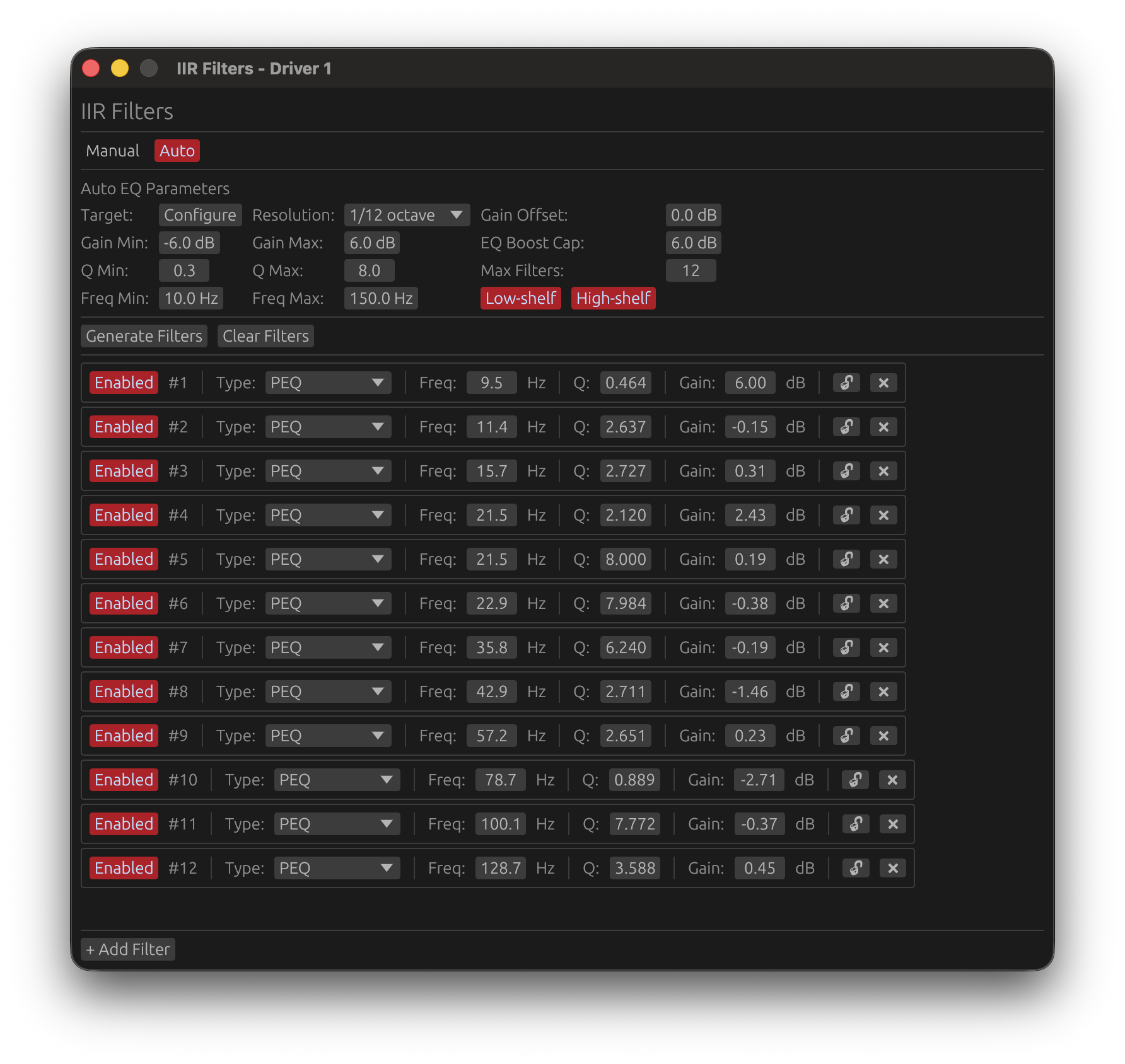
IIR Filter Tabs
The IIR window has two tabs:
Manual Tab
Design custom IIR filter chains with up to 50 filters.
Add Filter: Click ➕ Add Filter button
Remove Filter: Click ❌ button next to filter
Available Filter Types:
- Peak/Notch: Parametric EQ (boost/cut at specific frequency)
- Low Shelf: Boost/cut below shelf frequency
- High Shelf: Boost/cut above shelf frequency
- Low-Pass: Frequency-selective attenuation (high frequencies)
- High-Pass: Frequency-selective attenuation (low frequencies)
- All-Pass: Phase adjustment without magnitude change
Filter Parameters:
Frequency:
- Center frequency for Peak/Notch
- Cutoff frequency for LP/HP/Shelves
- Corner frequency for All-Pass
Gain (dB):
- Boost (+) or cut (-) amount
- Only for Peak/Notch and Shelving filters
- Range: -40 to +40 dB
Q Factor:
- Filter bandwidth/sharpness
- Higher Q = narrower bandwidth
- Typical range: 0.5 to 20
- Low Q (0.5-2): Wide, gentle curves
- Medium Q (2-5): Standard parametric EQ
- High Q (10-20): Narrow notches for resonance control
Order (LP/HP only):
- Filter slope steepness
- Range: 1 to 10 (depending on filter type)
- Each order adds 6 dB/octave slope
Pass Type:
- Low-Pass, High-Pass: Frequency-selective filtering
- Peak/Notch: Standard parametric EQ
Locked Filters (🔒):
Individual filters can be locked to preserve them during operations:
- Lock toggle: Click the 🔓/🔒 icon next to any filter to lock/unlock it
- Protected from Clear: Locked filters are not deleted when clicking “Clear Filters”
Use Cases:
- Lock protective filters (high-pass, low-pass) to preserve them when clearing other filters
- Preserve manually tuned filters when experimenting with different EQ approaches
- Protect critical filters (driver protection, subsonic filters) from accidental deletion
Auto Tab
Automatically generated equalization with manual control.
Adding Filters:
- Click ➕ Add Filter to manually add filters in Auto EQ tab
- Add protective filters (high-pass, low-pass, notches) before running Auto EQ
- Lock them with 🔒 icon to preserve during Auto EQ generation
Manual Editing:
- All filters in Auto EQ tab are editable (frequency, gain, Q)
- Adjust auto-generated filters directly without cloning
- Lock important filters to prevent removal during regeneration
Generate Auto EQ:
- Click Generate to automatically create corrective filters
- Auto EQ respects locked filters (integrates HP/LP into target curve)
- Unlocked filters are replaced with new auto-generated corrections
Copy to Manual:
- Click Clone from Auto EQ to copy the entire filter set to Manual tab
- Useful for preserving a working Auto EQ configuration while experimenting in Manual
Auto-generate (requires license)
- Enable the Auto-generate toggle to automatically re-generate filters whenever any parameter in the Auto EQ tab changes — frequency range, gain limits, resolution, shelves, etc.
- When first activated, a generation is immediately triggered with the current parameters
- Only parameter changes within the Auto EQ tab trigger regeneration; changes in the Manual tab or other driver settings have no effect
- Changing the target curve does not trigger auto-generation. To apply a new target curve, click Generate Filters manually or change any parameter in the Auto EQ tab after selecting the new curve
🔑 License required: The Auto-generate toggle requires a valid LinFIR license. Without a license, it is disabled and greyed out.
Target curve overlay
When the IIR filter window is open and in the foreground with the Auto EQ tab selected, the configured target curve is displayed as a blue overlay directly on the frequency response graph. The curve is level-matched to the driver’s smoothed response over the configured frequency range, and truncated to [Freq Min, Freq Max]. It disappears automatically when the IIR window is sent to the background.
Auto EQ Parameters
When you click Generate in the Auto EQ tab, the optimizer uses the following parameters to create corrective filters:
Gain Offset:
- Range: -20 to +20 dB
- Default: 0 dB
- Purpose: Adjusts the overall target level before EQ optimization
- Use case: Compensate for overall system level shifts without changing filter gains
Gain Min / Gain Max:
- Range: -20 to +20 dB
- Default: -6 to +6 dB
- Purpose: Limits the boost/cut range for each individual filter
- Use case: Prevent excessive corrections that could cause clipping or sound unnatural
EQ Boost Cap:
- Range: 0 to +20 dB
- Default: 6 dB
- Purpose: Soft-clips the correction target to prevent filter stacking at the same frequency
- Use case: Set lower values (e.g., 4 dB) for more conservative corrections
Q Min / Q Max:
- Range: 0.1 to 20.0
- Default: 0.3 to 8.0
- Purpose: Controls the bandwidth/sharpness of generated filters
- Use case: Lower Q = wider corrections, higher Q = narrow notches for resonances
Max Filters:
- Range: 1 to 30
- Default: 12
- Purpose: Maximum number of filters to generate (including shelves if enabled)
- Use case: More filters = more precise correction, but more phase impact
Freq Min / Freq Max:
- Range: 10 to 22,000 Hz
- Default: 20 to 20,000 Hz
- Purpose: Defines the frequency range for filter placement and correction
- Important: Auto EQ applies a quarter-octave taper (1/4 octave) above and below these frequency limits to ensure smooth transitions without discontinuities in the correction
- How the taper works:
- Below
Freq Min: Correction weight gradually reduces from 100% atFreq Minto 0% atFreq Min / 2^(1/4)(quarter-octave below) - Above
Freq Max: Correction weight gradually reduces from 100% atFreq Maxto 0% atFreq Max * 2^(1/4)(quarter-octave above) - Outside taper zones: No correction applied (weight = 0%)
- Below
- Use case: Focus correction on the driver’s operating band, exclude problematic regions (e.g., below resonance, room modes, or above useful bandwidth)
Low Shelf / High Shelf:
- Toggle: Enable/disable shelf filters
- Purpose: Allow AutoEQ to include shelving filters for broad tonal adjustments
- Use case: Enable for better overall tonal balance, disable for peaking-only corrections
Resolution:
- Options: 1/48, 1/24, 1/12, 1/6, 1/3 octave
- Default: 1/12 octave
- Purpose: Smoothing applied to the current response before optimization
- Use case: Higher smoothing (1/3 oct) = broader corrections, lower smoothing (1/48 oct) = more detailed corrections
IIR Filter Applications
Parametric EQ (Peak/Notch):
- Boost/cut specific frequencies
- Correct narrow resonances or notches
- Fine-tune response after FIR correction
Shelving Filters:
- Broad treble/bass adjustments
- Tilt EQ for overall tonal balance
- Baffle step compensation
- Psychoacoustic tuning
Notch Filters:
- Suppress driver resonances
Low-Pass/High-Pass:
- Additional crossover filtering (complements FIR)
- Subsonic/ultrasonic filtering
All-Pass:
- Phase correction without affecting magnitude
- Time alignment adjustments
- Advanced multi-driver phase matching
IIR Best Practices
-
Use sparingly:
- Fewer filters = cleaner phase response
- Each biquad adds phase rotation
- Prefer FIR correction for broad magnitude shaping
-
Narrow adjustments:
- IIR excels at narrow peaks/notches
- Use Q > 5 for resonances
- Use Q < 2 for broad tonal adjustments
-
Check phase impact:
- View phase plot when adding IIR filters
- High-Q filters create significant phase rotation
- Consider if phase impact is acceptable
-
Combine with FIR:
- FIR correction for broad trends (1/3 to 1/6 oct smoothing)
- IIR filters for narrow resonances and fine details
- Best of both worlds
Driver Adjustments
Polarity Inversion
Toggle: Polarity button
Inverts the driver’s signal (180° phase shift across all frequencies).
Use cases:
- Correct out-of-phase drivers
- Optimize multi-driver summation (especially for dipole/bipole designs)
- Fix inverted wiring
- Align asymmetric crossovers
How to check:
- Observe step response: positive step should have initial positive rise
- Check summed magnitude: in-phase drivers sum coherently (+6 dB), out-of-phase drivers cancel
Gain Adjustment
Range: -40 to +40 dB
Step: 0.1 dB
Default: 0 dB
Adjusts the driver’s output level.
Use cases:
- Compensate for driver sensitivity differences
- Set target SPL for each driver
- Balance multi-driver systems
- Fine-tune summed response
Time Delay
Range: 0.0 to 100.0 ms
Step: equivalent to 1 sample (depends on target sampling frequency)
Default: 0.0 ms
Adds pure time delay to the driver’s output.
Use cases:
- Align drivers physically offset from each other
- Compensate for acoustic center differences
- Time-align multi-way systems for coherent summation
- Correct for DSP processing delays
Calculation:
- Distance (m) to delay (ms): delay = distance / 0.343 m/ms
- Example: 10 cm offset = 0.291 ms delay
Delay Step Size:
- Automatically adjusted based on sample rate
- Higher sample rates allow finer delay precision
- Use fine adjustments for critical time alignment
FIR Compensation Delay
Range: 0.0 to 100.0 ms
Step: equivalent to 1 sample (depends on target sampling frequency)
Default: 0.0 ms
Additional delay applied only to the FIR filter chain, not the entire signal.
Purpose:
- Manual control over FIR filter impulse positioning
- Fine-tune FIR filter alignment when Auto Causal Alignment is disabled
- Shift FIR maximum to optimal crop window position
Use case: When combining multiple causal FIR filters, the impulse maximum may shift. FIR Compensation Delay allows manually repositioning the combined FIR response to avoid truncation. It is not the primary timing alignment tool—use the Time Delay feature for that.
Recommendation: Use Auto Causal Alignment unless you need precise manual control.
Processing Chain Summary
The complete driver processing chain:
-
Raw Impulse Response
- Loaded via IR Management window
- Windowed with configurable start/stop times
-
FIR Crossover Filters
- High-pass filter (if enabled)
- Low-pass filter (if enabled)
- Applied in time domain
-
FIR Correction Filter
- Magnitude correction (if enabled)
- Phase correction (if enabled)
- Applied in time domain
-
Combined FIR Filters
- All FIR filters convolved into single impulse response
- Cropped to configured tap length
- Causality interpolation applied
-
IIR Filtering
- Cascaded biquad sections
- Applied in time domain (as SOS transfer function)
-
Driver Adjustments
- Polarity inversion (if enabled)
- Gain adjustment
- Time delay
-
Final Output
- Processed driver response
- Summed with other drivers for system response
💡 Visualising filter impact: When a filter window (LP, HP, correction FIR, or IIR) is open for a driver, LinFIR can overlay a dashed pre-filter curve on the frequency, phase, and group delay graphs. This shows the driver response at step 1 (after windowing, before any filtering), letting you see exactly how much correction a filter is applying without switching views. Enable this in Settings → Graphs → Response Overlays → Show raw response when filter windows are open (requires a valid license).
Workflow Recommendations
Starting a New Driver
- Load impulse response via Manage IR
- Configure windowing to isolate direct sound
- Set filter length (512-4096 taps for most designs)
- Add FIR crossover (LP/HP) if needed
- Apply FIR correction (start conservative: 1/6 oct smoothing, 12 dB max gain)
- Check summed response, adjust gain/delay for coherent summation
- Add IIR filters for fine-tuning (narrow resonances, shelves)
- Optimize causality if latency is critical
- Export filters for DSP deployment
Multi-Way Design
- Load all driver IRs (woofer, midrange, tweeter)
- Set crossover frequencies based on driver capabilities
- Apply complementary crossovers (e.g., LR4 at matching frequencies)
- Check phase alignment and IR (step) summation in phase and IR (step) plots
- Adjust time delays to align acoustic centers
- Check summed magnitude for flat on-axis response
- Fine-tune with IIR for final voicing
- Verify step response for correct polarity and alignment
Keyboard Shortcuts
- Cmd+W / Ctrl+W: Close configuration windows (LP, HP, Correction, IIR)
- F: Switch to Filters display mode
- D: Switch to Drivers display mode
- U: Toggle wrapped/unwrapped phase
- C: Toggle time of flight rotation removal
See Keyboard Shortcuts for complete reference.
Related Documentation
- IR Management: Detailed impulse response loading and windowing
- System Processing: Global FIR correction and system-level processing
- Export: Exporting filters for DSP platforms
- Settings: Application-wide settings and defaults
System Processing
LinFIR provides global (system-wide) processing that applies corrections to the summed system response after all individual driver filters. This is available in both Loudspeaker Design and Room Calibration modes.
Global processing consists of two main components:
- Global FIR Correction Filter: Magnitude and phase correction of the summed system response
- Global IIR Filters: System-wide parametric EQ for room correction and final tuning
This page documents the global FIR correction filter. For global IIR filtering, see the corresponding section below.
Loudspeaker Design
Driver responses are summed to form the combined system response before correction.
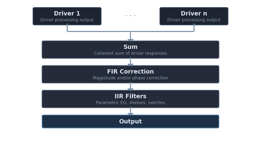
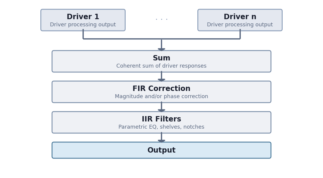
Room Calibration
Driver responses are averaged across measurement positions before correction.
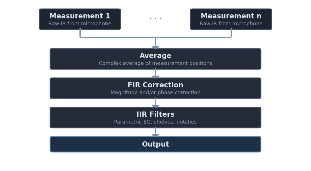
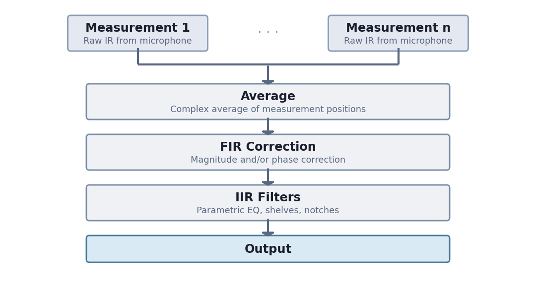
Global FIR Correction Filter
The Global FIR Correction Filter corrects the summed system response using FIR filters. It applies after all individual driver filters are combined, providing final system-level magnitude and phase correction.
Access the global FIR correction window from the Drivers/Measurements column (Global FIR button in the Global Filters section).
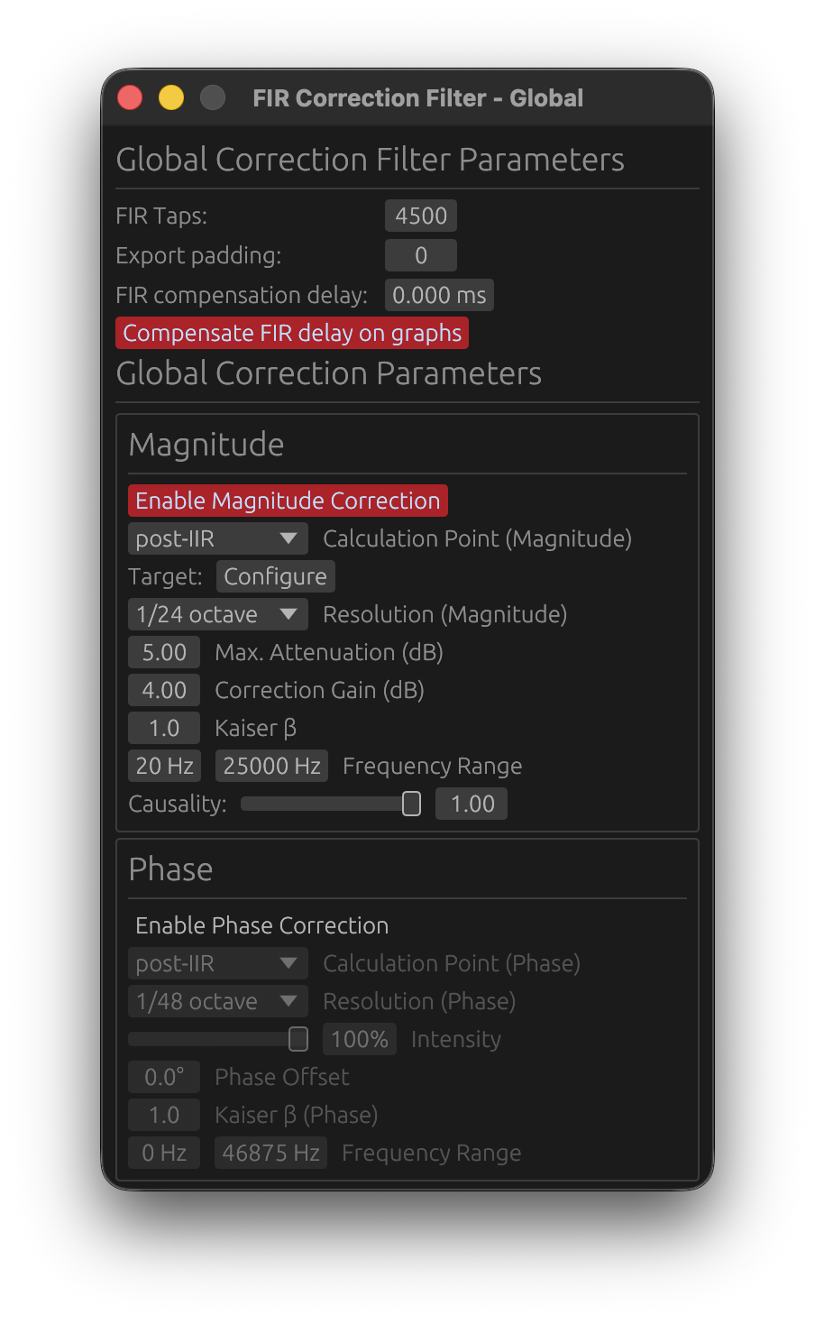
When to Use Global Correction
Loudspeaker Design Mode:
- Correct summed driver response/entire loudspeaker
- Align final system response to target curves (Flat, Harman, Custom)
- Compensate for baffle diffraction effects on the combined response
- Final system voicing and tuning
Room Calibration Mode:
- Room correction applied to the averaged measurements
- Correct combined room + speaker response
- Export global correction for integration into DSP processors
💡 Tip: Use global correction for overall tonal balance, and system-wide frequency response issues. Use per-driver correction (in Loudspeaker Design mode) for individual driver resonances, breakup modes, or response irregularities.
Global FIR Filter Length
FIR Taps
- Range: 32 to 65,536 taps
- Controls: the length (and thus frequency resolution) of the global FIR correction filter
How to choose:
- Higher tap counts → better low-frequency resolution, longer processing latency
- Lower tap counts → lower latency, reduced low-frequency precision
⚠️ Latency Note: The global FIR filter’s latency depends on tap count, magnitude causality, and phase correction:
- Causality = 1.0 (minimum-phase) + no phase correction: ~0 latency (impulse at t ≈ 0)
- Causality = 0.0 (linear-phase): ~
ntaps/2samples latency (impulse centered)- Phase correction enabled: adds latency regardless of causality (shifts impulse to center)
For low-latency applications, use Causality = 1.0 and disable phase correction.
Export Padding
- Range: 0 to 65,536 taps
- Purpose: Add zero-padding to the exported FIR filter files only
Export padding does not affect internal processing—it only extends the exported FIR coefficients with zeros. This is useful for:
- Meeting minimum FIR length requirements of external DSP platforms
- Aligning export formats across multiple filters
Example: If the global FIR filter is 4096 taps and you set export padding to 512, the exported file will contain 4608 coefficients (4096 actual + 512 zeros).
FIR Compensation Delay
- Range: -100 to +100 ms
- Purpose: Fine-tune the alignment of the global FIR filter in the processing chain
This parameter shifts the global FIR filter in time relative to the taps window.
Use Cases:
- Compensate for small timing misalignments introduced by FIR processing
- Adjust global FIR placement when mixing minimum-phase and linear-phase filters
💡 Tip: In most cases, leave this at 0 ms. Only adjust if you observe timing issues and ringing truncation in the impulse response.
Compensate FIR Delay on Graphs
- Toggle: Shift the impulse response left in plots to remove visual delay
When enabled:
- The impulse response plot shifts left by approximately
ntaps/2samples - The phase and group delay plots are also affected
- Exported filters are not modified
Purpose:
- Provides a clearer view of the aligned impulse response across drivers
- Useful for comparing driver responses without the visual offset from FIR latency
When to enable:
- When visually analyzing impulse alignment between drivers
- When comparing group delay and phase between the individual drivers and the sum
When to disable:
- When you need to see the true latency of the system
Magnitude Correction
The Magnitude Correction section corrects the frequency response (magnitude) of the summed system.
Enable Magnitude Correction
Toggle to enable/disable magnitude response correction independently from phase.
When disabled, magnitude correction settings are grayed out.
Reference (Magnitude)
- Options:
On-axisorListening Window - Default:
On-axis - Requires: A valid LinFIR license
Selects which response is used as input for computing the magnitude correction FIR filter.
On-axis:
- Uses the on-axis summed system response
- Standard behavior
Listening Window:
- Uses the spatial average of all polar measurements within ±30° horizontal and ±10° vertical as the correction input
- Corrects the tonal balance experienced across the listening zone, not just on-axis
- When selected, pre-IIR / post-IIR calculation point still applies normally
- Falls back to On-axis silently if fewer than 2 qualifying angles are available
💡 When to use Listening Window correction: When your listening position varies slightly off-axis (e.g., multiple listeners, wide seating arrangement), or when the speaker has significant directivity — the on-axis response may not be representative of what is actually heard. Correcting to a Listening Window average produces a more natural tonal balance across the sweet spot.
⚠️ Note: The Listening Window reference requires off-axis measurement data. Without at least 2 qualifying polar measurements, the option falls back to On-axis automatically.
Calculation Point (Magnitude)
- Options:
pre-IIRorpost-IIR - Purpose: Choose where to measure the system response for magnitude correction
pre-IIR:
- Measures the system before global IIR filters
- Corrects the summed driver response (FIR crossovers + driver FIR corrections + driver IIR)
- Use when you want to correct the raw driver summation before applying IIR EQ
post-IIR:
- Measures the system after global IIR filters
- Corrects the final system response (drivers + global IIR)
- Use for final system tuning or room correction that accounts for global IIR EQ
💡 Tip: For room calibration, use
post-IIRto correct the final room + speaker response. For loudspeaker design, usepre-IIRto correct driver interactions before applying global voicing EQ.
Target Curve
- Button:
Configure - Purpose: Select and configure the target curve for magnitude correction
Clicking Configure opens the Target Curve Window where you can:
- Select Flat or Harman as base curves
- Add inflection points and shape the curve
The magnitude correction FIR filter will match the response to this target curve.
See the Target Curves section in the documentation for details on curve types and customization.
Resolution (Magnitude)
- Options:
1/48 octave,1/24 octave,1/12 octave,1/6 octave,1/3 octave - Purpose: Control the smoothing applied to the magnitude correction
Lower fractions (e.g., 1/48 oct) → finer detail, corrects small ripples
Higher fractions (e.g., 1/3 oct) → broader smoothing, corrects only major trends
How to choose:
- Room correction: Use
1/6 octaveor1/3 octaveto avoid over-correcting room modes (which vary with position) - Loudspeaker design: Use
1/12 octaveor1/24 octavefor detailed driver correction
⚠️ Warning: Very fine smoothing (1/48 oct) can lead to excessive correction of measurement noise. Use with caution.
Max Attenuation
- Range: 0 to 30 dB
- Default: 10 dB
- Purpose: Limit the maximum attenuation (cut) applied by magnitude correction
This parameter “cuts from the top”—it limits how much the correction filter can reduce peaks in the frequency response.
Why limit attenuation?
- Prevents excessive cuts that waste headroom
- Avoids over-correcting narrow resonances (which may not be audible)
- Maintains system efficiency
Example:
- If the system has a +15 dB peak at 200 Hz and Max Attenuation is set to 10 dB, the correction will cut only 10 dB (leaving a +5 dB peak)
Recommended values:
- Room correction: 10–15 dB (room modes can be large)
- Loudspeaker design: 6–10 dB (driver peaks are typically smaller)
Correction Gain
- Range: -20 to +20 dB
- Default: 4 dB
- Purpose: Add gain to the correction filter to compensate for attenuation and maintain system level
Magnitude correction typically attenuates peaks, which reduces overall loudness. Correction Gain adds a fixed boost to restore the level.
How to choose:
- Set Correction Gain to approximately match the average attenuation applied
- For example, if the correction cuts ~4 dB on average, set Correction Gain to +4 dB
💡 Tip: Adjust Correction Gain by observing the final system level after correction. Too much gain can cause clipping or driver damage; too little leaves the system quieter than before.
Kaiser β (Magnitude)
Range: 0.0 to 50.0
Default: 8.0
Kaiser windowing parameter for the magnitude correction FIR filter.
Effect:
- Lower values (3-5): Sharper correction BUT may increase ringing
- Moderate values (6-10): Good balance between precision and ringing suppression
- Higher values (12-20): Smoother correction, reduced ringing, but less precise
Recommendation: Start with default 8.0, decrease to 1-2 if ringing is not problematic.
Frequency Range (Magnitude)
- f_min (minimum frequency): Starting point for magnitude correction
- f_max (maximum frequency): Ending point for magnitude correction
- Fade-in/Fade-out: Smooth transitions at the boundaries
Purpose: Limit magnitude correction to a specific frequency range.
Example:
- Set
f_min = 40 Hzandf_max = 12,000 Hzto correct only mid-bass through mid-treble, leaving deep bass and extreme treble unaffected
💡 Tip: Avoid correcting frequencies outside the measurement’s reliable range. Measurement noise dominates at the extremes.
Causality (Magnitude)
Range: 0.0 (linear-phase) to 1.0 (minimum-phase)
Default: 1.0 (minimum-phase)
Controls the phase characteristic of the magnitude correction filter.
- 0.0 (Linear-phase): Symmetric pre- and post-ringing, constant group delay
- 1.0 (Minimum-phase): No pre-ringing, all energy is causal, variable group delay
Typical choice: 1.0 (minimum-phase) to avoid pre-ringing artifacts.
Why minimum-phase is preferred: Most acoustic and electronic systems are minimum-phase (magnitude and phase are coupled via Kramers-Kronig relations). Correcting magnitude with a minimum-phase filter automatically corrects the associated phase deviation, providing physically accurate correction. Use 0.0 (linear-phase) only if you specifically need constant group delay with a non-flat target curve and can tolerate pre-ringing.
Phase Correction
The Phase Correction section corrects the group delay and phase response of the summed system.
Enable Phase Correction
Toggle to enable/disable phase response correction independently from magnitude.
🚫 Non-anechoic measurements: phase correction is strongly discouraged
Phase correction requires clean, accurate phase data. In-room measurements contain reflections, room modes, and position-dependent artifacts that pollute the phase response. Applying phase correction to such data produces unpredictable — and often worse — results.
Only use phase correction with anechoic or near-anechoic measurements (e.g., measurements gated to remove reflections, or made in an anechoic chamber). For in-room measurements, restrict correction to magnitude only.
Exception — Room Calibration mode with spatially averaged measurements: When the corrected response is the result of averaging several measurements taken at different listening positions, the influence of room modes and position-dependent reflections is drastically reduced. In this specific case, phase correction becomes more acceptable, as the averaged phase data is significantly less polluted than any single-point measurement.
Even so, spatial averaging is not a perfect substitute for anechoic conditions. A final verification measurement and critical listening session are recommended to confirm that no audible artifacts or regressions have been introduced by the phase correction.
⚠️ Critical Limitation: Phase Correction vs. Low Latency
You cannot have both near-zero latency FIR filters AND active phase correction. This is a fundamental limitation, not a software bug.
Why this incompatibility exists:
Even if you configure your FIR magnitude correction with causality = 1.0 (minimum-phase, low latency), which positions the FIR impulse peak near t=0 (left-aligned), enabling phase correction will shift the combined FIR impulse peak to the center (around ntaps/2), introducing significant latency.
The reason is fundamental:
- Phase correction = temporal correction: Phase distortion is fundamentally a time-domain problem (different frequencies arriving at different times)
- To correct temporal defects, you need time: The filter needs temporal “space” before and after the main impulse to reposition frequency components correctly
- This requires centering the impulse: Phase correction filters must have headroom both before (pre-ringing) and after (post-ringing) the main signal to perform time-domain manipulations
- Result: The combined FIR impulse peak moves from t≈0 (low latency) to t≈ntaps/2 (high latency)
Practical impact:
- Without phase correction: Causality=1.0 filters → impulse peak at t≈0 → latency ≈ 0 samples
- With phase correction enabled: Impulse peak moves towards t≈ntaps/2 → latency ≈ ntaps/2 samples (e.g., 2048 samples at 48kHz = 42.7ms)
Recommended approach:
- For low-latency applications (live sound, PA, monitoring): Use causality = 1.0 on crossover/magnitude filters, disable phase correction, accept phase as-is
- For high-fidelity applications (studio monitors, reference systems): Use causality = 0.0 on crossover, 1.0 on magnitude filters, enable phase correction if needed, accept the latency
- For hybrid approach: Use moderate causality (0.3-0.7) for reduced latency with some phase correction capability (but still expect significant latency when phase correction is active)
Calculation Point (Phase)
- Options:
pre-IIRorpost-IIR - Purpose: Choose where to measure the system response for phase correction
pre-IIR:
- Measures phase before global IIR filters
- Corrects driver phase interactions (crossover phase shifts, driver delays)
- Use when global IIR has minimal phase impact
post-IIR:
- Measures phase after global IIR filters
- Corrects final system phase (including IIR phase shifts)
- Use for complete system phase linearization
💡 Tip: Phase and magnitude correction can use different calculation points. For example, use
pre-IIRfor magnitude (correct drivers) andpost-IIRfor phase (linearize final system).
Resolution (Phase)
- Options:
1/48 octave,1/24 octave,1/12 octave,1/6 octave,1/3 octave - Purpose: Control the smoothing applied to phase correction
Same principle as magnitude resolution:
- Finer smoothing (1/48 oct) → corrects small phase variations
- Coarser smoothing (1/3 oct) → corrects only major phase trends
Recommended values:
- Room correction: 1/6 or 1/3 octave
- Loudspeaker design: 1/12 or 1/24 octave
Intensity
- Range: 0% to 100%
- Default: 100%
- Purpose: Control the strength of phase correction
100%: Full phase correction (matches measured phase to target)
0%: No phase correction
50%: Half-strength correction (blend between measured and target phase)
Use Cases:
- Reduce intensity (e.g., 70–80%) if full phase correction introduces audible artifacts
- Use partial correction to preserve some driver phase characteristics
💡 Tip: Start with 100% and reduce intensity if the correction sounds unnatural.
Phase Offset
Range: -180° to +180°
Default: 0°
Phase offset applied to the filter’s phase response.
Purpose: Controls the symmetry of the impulse response by adjusting the phase offset. This allows fine-tuning the balance between pre-ringing and post-ringing in the time-domain response.
How it works:
- 0°: Default even symmetric behavior
- Positive/Negative offset: Shifts impulse response characteristics towards odd symmetry
Use case: Advanced parameter for optimizing impulse response symmetry in multi-driver systems.
Recommendation: Leave at 0° unless you have specific symmetry requirements and understand impulse response trade-offs.
Kaiser β (Phase)
Range: 0.0 to 50.0
Default: 1.0
Kaiser windowing parameter for the phase correction FIR filter.
Effect:
- Lower values (1-5): Less aggressive windowing — the correction filter’s oscillations (pre- and post-ringing) are preserved more fully, allowing accurate phase correction
- Moderate values (6-10): Balanced windowing — trade-off between accuracy and artifact suppression
- Higher values (12-20): Aggressive windowing — strongly attenuates pre- and post-ringing, which can introduce magnitude deviations if correction energy is clipped
When to adjust:
- If the guard warning appears (the auto-guard has already narrowed the Start/End Frequencies as far as it can): decrease Kaiser β — see Phase Correction Magnitude Artifacts
- If phase correction creates excessive ringing, increase Kaiser β
Recommendation: Start with default 1.0. If the guard warning still appears after its automatic frequency adjustments, try reducing β toward 0.
Frequency Range (Phase)
- Start Frequency: Starting point for phase correction
- End Frequency: Ending point for phase correction
Purpose: Limit phase correction to a specific frequency range.
Use Cases:
- Avoid correcting phase at frequencies where group delay measurements are unreliable
- Avoid correcting phase outside speaker’s frequency response
- Reduce magnitude artifacts: low frequencies require the longest correction filters; the auto-correction guard raises the Start Frequency automatically when artifact warnings occur — see Phase Correction Magnitude Artifacts for a full explanation and resolution procedure
Global IIR Filtering
In addition to global FIR correction, LinFIR provides Global IIR Filters for system-wide parametric EQ.
When to Use Global IIR
- Room correction EQ: Parametric filters to address specific room modes
- Final system tuning: Overall tonal balance adjustments (bass/treble tilt, voicing)
- Low taps count: IIR filters require less processing power, allowing easier low end correction with small DSP processors
💡 Tip: Use global IIR for low end corrections and global FIR for high frequencies correction.
Access Global IIR Window
Access the global IIR window from the Drivers/Measurements column (Global IIR button in the Global Filters section).
Manual vs. Auto EQ Tabs
The Global IIR window has two tabs, identical to the per-driver IIR system:
Manual Tab:
- Manually add/edit parametric filters (PEQ, low shelf, high shelf, etc.)
- Full control over frequency, gain, Q
- Lock individual filters to prevent Auto EQ from modifying them
Auto EQ Tab:
- Automatically generates IIR filters to match the system to a target curve
- Same parameters as driver Auto EQ:
- Gain Offset: Adjust overall target level
- EQ Boost Cap: Prevent excessive boost
- Frequency range, Q range, Filter count
- Auto-generate toggle (requires license): see Auto-generate in the driver IIR documentation — same behaviour applies here; note that changing the target curve does not trigger auto-generation
Target curve overlay
When the Global IIR window is open and in the foreground with the Auto EQ tab selected, the configured target curve is displayed as a blue overlay directly on the frequency response graph. The curve is level-matched to the summed system response over the configured frequency range, and truncated to [Freq Min, Freq Max]. It disappears automatically when the window is sent to the background.
Auto EQ (Global)
Global Auto EQ works on the summed system response after driver processing:
- Measures the final system (drivers + global FIR + global IIR)
- Generates IIR filters to match the selected target curve (Flat, Harman, Custom)
- Applies to the entire system (not per-driver)
Reference
- Options:
On-axisorListening Window - Default:
On-axis - Requires: A valid LinFIR license
Selects which response is measured to generate the Auto EQ filters.
On-axis:
- Uses the on-axis summed system response
- Standard behavior
Listening Window:
- Uses the spatial average of all polar measurements within ±30°H / ±10°V as the response being equalized
- Optimizes the IIR filter shape to correct the Listening Window response towards the target curve
- The level reference (absolute dB anchor) is always taken from the on-axis response, regardless of this setting — this prevents a net gain offset from being introduced by the LW averaging
- Falls back to On-axis if fewer than 2 qualifying angles are available
💡 Tip: Using Listening Window for Auto EQ is particularly effective when the speaker has audible directivity variations within ±30°. The generated filters will address tonal imbalances that are present across the listening zone but may not be visible on the on-axis curve alone.
Use Cases:
- Room correction: Auto EQ generates filters to correct room + speaker response
- Final voicing: Quick tonal adjustments without regenerating FIR filters
Locked Filters (🔒):
Individual filters can be locked to preserve them during operations:
- Lock toggle: Click the 🔓/🔒 icon next to any filter to lock/unlock it
- Protected from Clear: Locked filters are not deleted when clicking “Clear Filters”
- Protected from Auto EQ: Locked filters are not removed when regenerating Auto EQ
- Integration into Auto EQ:
- locked filters are integrated into the Auto EQ target curve
- The optimizer respects their frequency response instead of trying to compensate
Use Cases:
- Set a protective high-pass filter, lock it, then let Auto EQ optimize the rest
- Lock a low-pass filter for driver protection while auto-correcting midrange
- Preserve manually tuned filters while regenerating Auto EQ corrections
- Combine manual protective filters with automatic room correction
Example Workflow:
- Switch to Auto EQ tab
- Add protective filters (e.g., -24 dB/oct HP at 60 Hz, room mode notches) using ➕ Add Filter
- Lock them using the 🔒 icon
- Configure target curve (Flat, Harman, Custom)
- Click “Generate” to run Auto EQ optimization
- Review and adjust: Edit any auto-generated filter directly (frequency, gain, Q)
- Lock refined filters: Lock manually adjusted filters to preserve them
- Iterate: Regenerate Auto EQ as many times as needed—locked filters stay in place
- Result: Auto EQ creates corrective filters while respecting locked protective filters
📖 For detailed Auto EQ parameter descriptions, see the Driver Processing page (Auto EQ section). Global Auto EQ uses identical parameters.
Workflow Recommendations
Loudspeaker Design Mode
- Design individual driver filters (FIR crossovers, FIR corrections, IIR EQ)
- Verify summed system response (check for phase cancellations, comb filtering)
- Apply global FIR correction if needed:
- Correct driver interaction issues (dips, peaks from crossover summing)
- Match system to target curve (Flat, Harman)
- Add global IIR filters for final voicing (bass/treble tilt, room-specific adjustments)
- Export filters for DSP platform
Room Calibration Mode
- Measure room response at listening position
- Apply global FIR correction:
- Set resolution to 1/6 or 1/3 octave (avoid over-correcting room modes)
- Limit frequency range (e.g., 500–18,000 Hz)
- Set Max Attenuation to 10–15 dB
- Add global IIR filters for specific room modes (parametric notches)
- Re-measure and iterate if needed
- Export global correction filters for room DSP processor
💡 Best Practice: In room calibration mode, avoid excessive correction of room modes and deep nulls. Boosting these regions by more than 6-10 dB risks clipping, increased distortion, driver overexcursion, and potential damage. Use acoustic treatment for problematic modes instead of EQ.
Related Documentation
- Driver Processing: Per-driver FIR/IIR filtering (loudspeaker design mode)
- Settings: Application-wide filter processing defaults
- Target Curves: Configuring Flat, Harman, and Custom curves
- Export: Exporting filters for DSP platforms (input FIR vs. output FIR)
Summary
Global FIR Correction provides system-level magnitude and phase correction for:
- Loudspeaker Design: Correcting summed driver interactions and final system voicing
- Room Calibration: Correcting room + speaker response at the listening position
Key Features:
- Independent magnitude and phase correction with separate calculation points (pre-IIR/post-IIR)
- Adjustable resolution, frequency range, and causality for flexible correction strategies
- FIR compensation delay and graph compensation for fine-tuning alignment and visualization
Global IIR Filtering complements FIR correction with:
- Manual parametric EQ for precise corrections
- Auto EQ for automatic target curve matching
- Locked filters for hybrid manual/automatic workflows
Use global processing after per-driver processing to achieve final system performance targets.
Target Curves
Target curves define the desired frequency response for FIR correction and Auto EQ optimization. LinFIR provides built-in curves (Flat, Harman) and supports fully customizable user-defined curves.

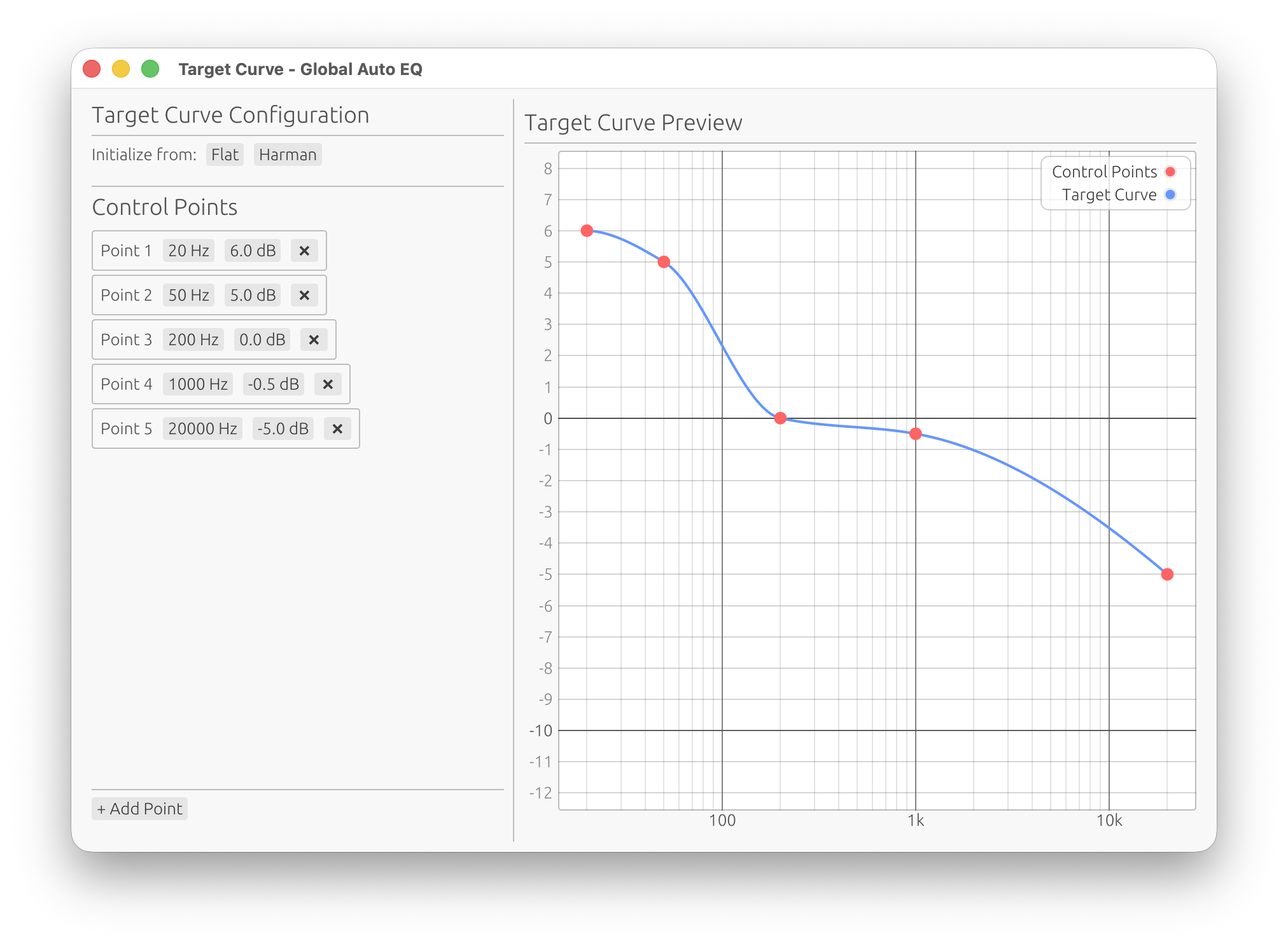
Target curves are used by:
- FIR Correction filters (per-driver and global)
- Auto EQ (per-driver and global IIR optimization)
Each filter type has its own independent target curve configuration.
Accessing Target Curve Configuration
Target curve windows are accessed from configuration buttons in the corresponding filter windows:
Per-Driver:
- FIR Correction: Driver → FIR Correction → Magnitude Correction section → Configure button
- Auto EQ: Driver → IIR Filters → Auto EQ tab → Target Curve section → Configure button
Global:
- Global FIR Correction: Global FIR → Magnitude Correction section → Configure button
- Global Auto EQ: Global IIR → Auto EQ tab → Target Curve section → Configure button
Built-in Target Curves
Import / Export
Control points can be saved to and loaded from plain-text files using the 📂 Import and 💾 Export buttons, located just below the Initialize from buttons in the toolbar.
File Format
A simple two-column text file:
# LinFIR target curve
# Frequency (Hz)	Gain (dB)
20.00	0.00
200.00	-2.50
1000.00	-4.00
20000.00	-8.00
Rules:
- One point per line:
frequency<sep>gain - Separator: tab, space or comma (mixed is fine)
- Lines starting with
#are ignored (comments) - Empty lines are ignored
- Decimal separator:
.(a,is also accepted and converted automatically) - Frequency must be strictly positive; gain can be any finite value
- At least 2 valid points are required for a successful import
- On import, points are sorted by ascending frequency automatically
Import (📂)
- Click 📂 Import
- Select a
.txtfile in the file picker - LinFIR parses the file and replaces the current control points
- The target curve preview updates immediately
If the file contains fewer than 2 valid points the import is silently ignored — the current points are preserved.
Export (💾)
- Click 💾 Export
- Choose a destination and file name (
.txtextension is added automatically if omitted) - The file is written with a commented header and tab-separated columns
Exported files can be shared between different target curve windows or projects, and edited with any text editor or spreadsheet application.
Flat Curve
Description: 0 dB gain across all frequencies (20 Hz to 20 kHz)
Use Cases:
- Anechoic measurements requiring no psychoacoustic compensation
- Verification/troubleshooting (no tonal bias)
- Starting point for custom curves
Initialization:
- Click Flat button
- Creates 2 control points: (20 Hz, 0 dB) and (20 kHz, 0 dB)
Harman Target Curve
Description: Psychoacoustically optimized frequency response based on Harman research
Curve Shape:
- +6 dB at 20 Hz: Enhanced deep bass presence
- +5 dB at 50 Hz: Bass warmth
- 0 dB at 200 Hz: Neutral lower midrange
- -0.5 dB at 1 kHz: Slight midrange dip (reference frequency)
- -5 dB at 20 kHz: Treble roll-off (reduces harshness)
Use Cases:
- In-room listening: Compensates for typical room gain and psychoacoustic preferences
- Room calibration: Starting point for subjective tuning
Initialization:
- Click Harman button
- Creates 5 control points with Harman curve shape
Customization:
- Adjust bass tilt by modifying low-frequency points
- Adjust treble slope by changing high-frequency points
- Add intermediate points for detailed shaping
⚠️ Critical: Max. Attenuation vs. Curve Amplitude
FIR correction filters work primarily by attenuation (cutting peaks). The Max Attenuation parameter must be large enough to accommodate the amplitude of the target curve within the configured frequency range.
Example (full Harman curve, 20 Hz - 20 kHz): The default Harman curve has an amplitude of 11 dB (from +6 dB at 20 Hz to -5 dB at 20 kHz). If you set Max Attenuation to only 6 dB, the FIR filter cannot apply the full curve—specifically, the treble roll-off (-5 dB at 20 kHz) will not be applied.
Example (limited range, 200 Hz - 20 kHz): If you set Frequency Range from 200 Hz to 20 kHz, the effective amplitude is only 5 dB (from 0 dB at 200 Hz to -5 dB at 20 kHz). In this case, Max Attenuation ≥ 5 dB is sufficient.
Rule: Set Max Attenuation ≥ curve amplitude within f_min to f_max.
- Calculate amplitude: Find max and min gain within your configured frequency range
- Harman (20 Hz - 20 kHz): Use Max Attenuation ≥ 11 dB (recommend 12-15 dB)
- Harman (200 Hz - 20 kHz): Use Max Attenuation ≥ 5 dB (recommend 6-8 dB)
- Custom curves: Calculate max - min within your f_min/f_max range
Applies to: FIR Correction filters (per-driver and global). Auto EQ uses IIR filters (can boost and cut freely).
Custom Target Curves
Create fully custom target curves with unlimited control points.
Control Points
Each control point defines a (frequency, gain) pair:
Frequency:
- Range: 1 Hz to 21,000 Hz
- Log-scale distribution recommended (e.g., 20, 50, 100, 200, 500, 1k, 2k, 5k, 10k, 20k Hz)
- Drag value to adjust
Gain:
- Range: -20 dB to +20 dB
- Positive values = boost, negative = cut
- Drag value to adjust
Minimum Points: 2 (required for interpolation)
Adding Points
- Click + Add Point button
- New point created at 1 kHz, 0 dB
- Adjust frequency and gain as needed
Removing Points
- Click ❌ button next to the control point
- Cannot remove if only 2 points remain (minimum requirement)
Curve Interpolation
LinFIR automatically interpolates between control points to create a smooth curve:
Interpolation Process:
- Generate 5,000 log-spaced frequencies across the full range
- Log interpolation between user control points onto these 5,000 frequencies
- Linear interpolation from 5,000 points to target frequencies (filter FFT bins)
Result: Smooth, natural curve without artifacts even with few control points
Preview: Real-time graph shows interpolated curve (blue line) and control points (red dots)
Target Curve Preview Graph
The right panel shows a real-time preview of the target curve.
Elements:
- Blue line: Final interpolated target curve (used by correction algorithms)
- Red dots: User-defined control points
Axes:
- X-axis: Frequency (Hz, logarithmic scale)
- Y-axis: Gain (dB, linear scale)
Auto-scaling: Y-axis automatically adjusts to fit data range
Workflow Recommendations
Creating a Custom Curve from Scratch
- Click Flat to start with a neutral baseline
- Add control points at key frequencies:
- 20 Hz: Deep bass level
- 50-100 Hz: Bass warmth
- 200-500 Hz: Lower midrange body
- 1 kHz: Reference point (usually 0 dB or slightly negative)
- 2-5 kHz: Presence region
- 10 kHz: Air/sparkle
- 20 kHz: Extreme treble roll-off
- Adjust gains to shape desired response
- Preview in graph and test with measurements
Modifying Harman Curve
- Click Harman to load default curve
- Adjust existing points:
- Reduce 20-50 Hz gains for less bass
- Increase 20 kHz gain for more treble extension
- Add points at 2-5 kHz for presence adjustment
- Use as starting point for room-specific tuning
Room Calibration Workflow
- Measure in-room response without any FIR or IIR EQ
- Start with Harman curve (accounts for typical room gain)
- Apply correction and re-measure
- Fine-tune target curve:
- Reduce bass points if room has excessive low-frequency gain
- Adjust treble roll-off based on room absorption
- Add notches at problematic room modes (if using Auto EQ)
- Iterate until subjectively satisfying
Loudspeaker Design Workflow
- Use Flat curve for anechoic FIR correction (individual drivers)
- Measure on-axis response and apply correction
- Verify off-axis response maintains reasonable shape
Best Practices
Control Point Placement
- Use logarithmic spacing: Match human auditory perception (e.g., 20, 50, 100, 200, 500 Hz…)
- Avoid excessive points: 5-10 points typically sufficient for smooth curves
- Anchor bass and treble: Always define endpoints (20 Hz, 20 kHz)
- Reference at 1 kHz: Many conventions use 1 kHz as 0 dB reference
Curve Shape Considerations
- Avoid steep transitions: Can cause ringing in FIR filters and excessive Q in Auto EQ
- Match measurement reliability: Don’t define detailed curve below measurement noise floor
- Account for driver capabilities: Don’t demand excessive bass from small drivers
- Psychoacoustic balance: Consider Fletcher-Munson curves at typical listening levels
FIR Correction: Max Attenuation vs. Curve Amplitude
Critical requirement for FIR correction filters:
FIR correction works primarily by attenuation (cutting peaks in the frequency response). The Max Attenuation parameter limits how much the filter can cut.
Problem: If the target curve has a large amplitude (difference between highest and lowest points), and Max Attenuation is set too low, the filter cannot apply the full curve shape.
Solution: Set Max Attenuation ≥ curve amplitude within the configured frequency range
Calculating Curve Amplitude:
- Find the highest gain in your target curve within f_min to f_max (configured Frequency Range)
- Find the lowest gain in your target curve within f_min to f_max
- Amplitude = highest - lowest within that range
Examples:
Harman curve, full range (20 Hz - 20 kHz):
- Highest: +6 dB at 20 Hz
- Lowest: -5 dB at 20 kHz
- Amplitude: 6 - (-5) = 11 dB
- Required: Max Attenuation ≥ 11 dB (recommend 12-15 dB)
Harman curve, limited range (200 Hz - 20 kHz):
- Highest: 0 dB at 200 Hz
- Lowest: -5 dB at 20 kHz
- Amplitude: 0 - (-5) = 5 dB
- Required: Max Attenuation ≥ 5 dB (recommend 6-8 dB)
Flat curve (any range):
- Amplitude: 0 dB (curve is flat)
- Any Max Attenuation works
Custom +10 dB bass, -8 dB treble, full range:
- Amplitude: 10 - (-8) = 18 dB
- Required: Max Attenuation ≥ 18 dB (recommend 20 dB)
What happens if Max Attenuation is too low:
- The filter clips the attenuation at the maximum value
- Parts of the curve are not applied (typically treble roll-off is lost)
- Result: Incomplete correction, unbalanced tonal response
Recommendation:
- Calculate amplitude only within your configured f_min/f_max range
- Add 1-3 dB margin above calculated amplitude
- Monitor corrected frequency response to verify full curve is applied
- If limiting frequency range (e.g., 200 Hz - 10 kHz), you may need much less Max Attenuation
💡 Tip: This only applies to FIR correction filters. Auto EQ uses IIR filters which can boost and cut freely, so this limitation does not apply.
Testing and Validation
- Preview before applying: Check interpolated curve makes sense
- Apply to measurement: Use with FIR correction or Auto EQ
- Measure result: Verify corrected response matches target
- Iterate: Refine target based on measurements and listening tests
Technical Details
Interpolation Algorithm
Step 1: Log-space interpolation
- Creates 5,000 log-spaced frequencies from minimum to maximum input frequency
- Uses logarithmic interpolation between user control points
- Preserves smooth transitions in log-frequency domain
Step 2: Linear resampling
- Resamples 5,000-point curve to target frequencies (FFT bins)
- Linear interpolation ensures smooth curve on target grid
- No artifacts or discontinuities
Result: High-quality curve suitable for both FIR convolution and IIR optimization
Frequency Range
- Minimum: 1 Hz (typically clamp to 20 Hz in practice)
- Maximum: 21,000 Hz (or Nyquist frequency, whichever is lower)
- Interpolation: Extends user points across full range
Gain Limits
- Range: -20 dB to +20 dB per control point
- No hard limit on curve: Interpolation can produce values outside this range between points
- Practical limit: Avoid extreme gains to prevent filter artifacts
Common Use Cases
Studio Monitoring
Target: Custom curve with gentle tilt (or modified Harman)
- Modern practice uses in-room curves rather than flat anechoic response
- Gentle treble roll-off (-1 to -3 dB at 20 kHz) reduces listening fatigue
- Slight bass lift (+1 to +3 dB below 100 Hz) compensates for room interaction
- Purely flat curves are rarely used in practice—can sound harsh and fatiguing
- Start with Harman and adjust to taste for extended listening sessions
Home Theater
Target: Harman curve (or modified)
- Preferred tonal balance for movies and music
- Accounts for room gain
- Adjust bass/treble tilt to taste
Hi-Fi Listening
Target: Custom curve based on Harman
- Start with Harman, adjust to preference
- Reduce bass if room is overly boomy
- Adjust treble based on speaker and room brightness
Car Audio
Target: Custom curve (elevated bass and treble)
- Compensate for road noise (boost bass and treble)
- Account for small cabin gain
- Highly subjective—tune by ear
Headphone Compensation
Target: Diffuse-field or Harman headphone curve
- Compensate for headphone frequency response
- Simulate speaker-like tonality
Related Documentation
- Driver Processing: FIR correction and Auto EQ using target curves
- System Processing: Global FIR correction and Auto EQ
Summary
Target curves define the desired frequency response for correction algorithms:
- Built-in curves: Flat (0 dB) and Harman (psychoacoustic optimized)
- Custom curves: Unlimited control points with automatic interpolation
- Independent configuration: Each FIR correction and Auto EQ has its own target
- Real-time preview: Interactive graph shows interpolated curve
Workflow:
- Open target curve window from filter configuration (Configure button)
- Initialize from Flat or Harman, or create custom
- Add/edit control points (frequency, gain)
- Import an existing curve from a text file, or export the current curve for reuse
- Preview interpolated curve in real-time
- Apply correction and measure results
- Iterate based on measurements and listening tests
Use target curves to shape your system’s tonal balance, compensate for room effects, and achieve your desired sound signature.
Spectrogram 🔒
License Required: The Spectrogram window requires a valid LinFIR license.
The Spectrogram visualises the time-frequency energy distribution of the impulse response as a 2-D colour map, making it easy to spot resonances, ringing, and temporal smearing that are difficult to see in a standard frequency response plot.
- Loudspeaker Design mode — shows the predicted sum impulse response for the currently selected angle (on-axis by default); when a non-zero angle is selected in the angle selector the spectrogram updates to reflect that off-axis response, and the window title shows the active angle (e.g. Spectrogram — Predicted Sum — +15°H +0°V)
- Room Calibration mode — shows the averaged measurement impulse response
Accessing the Spectrogram
Menu: View → Spectrogram
Keyboard shortcut: W
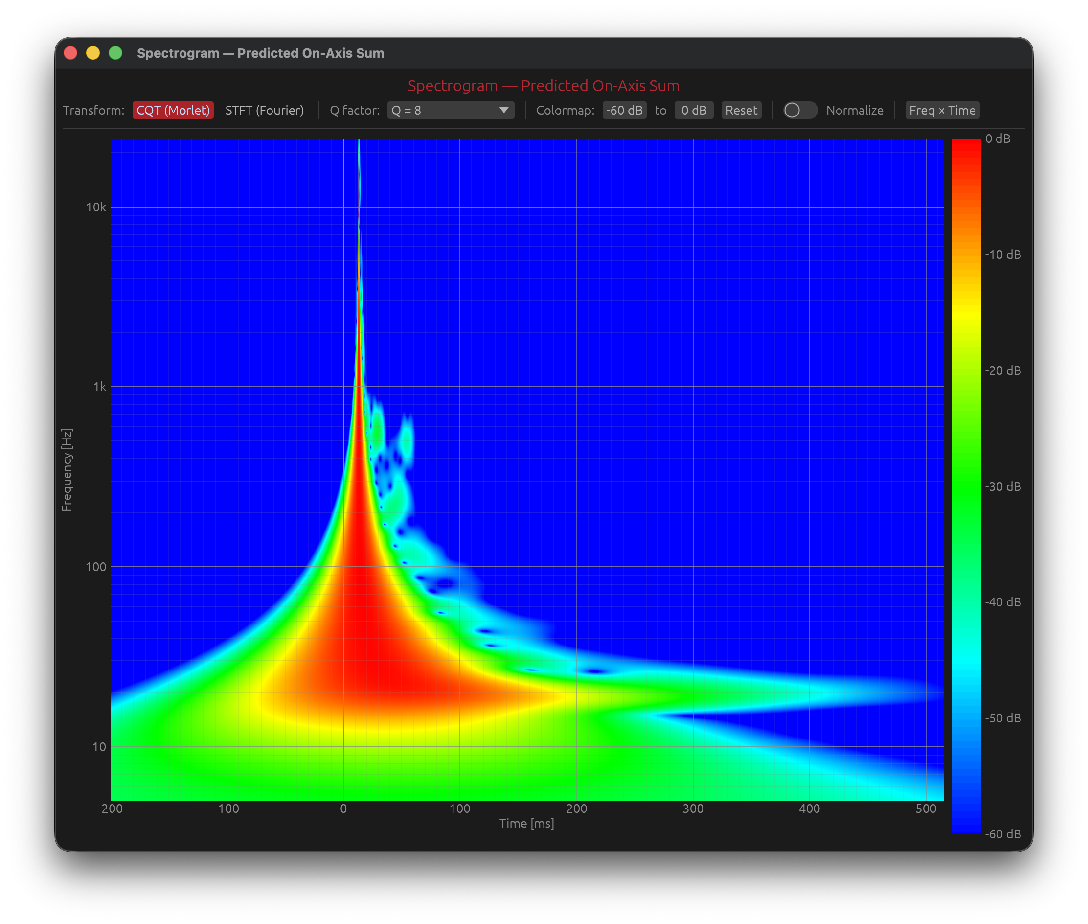
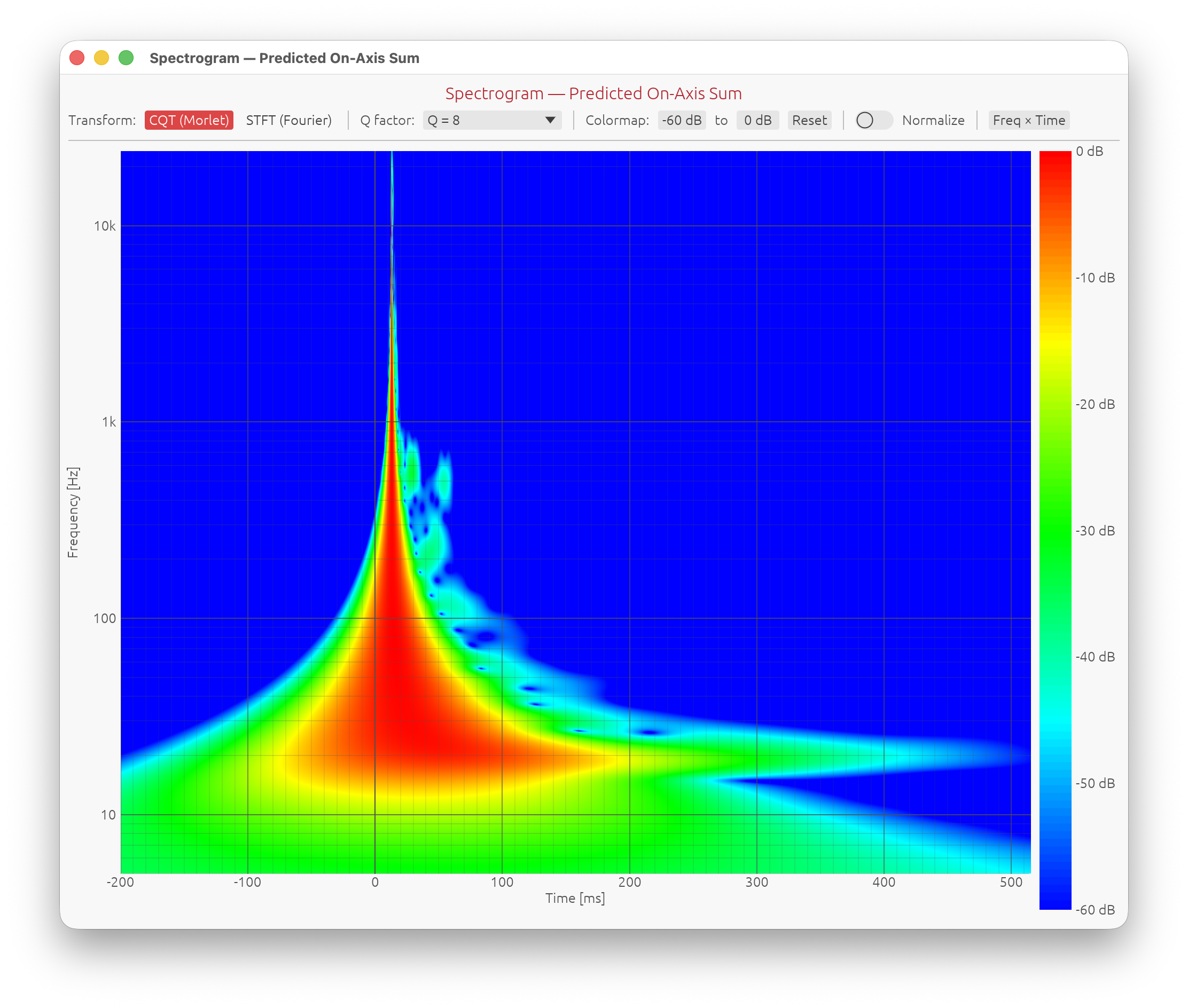
Layout
The window is divided into two panels:
- Main plot — the colour-mapped spectrogram
- Colorbar (right edge) — dB scale matching the current colormap range
A control bar above the plot exposes all parameters.
Controls
Transform Algorithm
Two algorithms are available, selectable via the CQT (Morlet) / STFT (Fourier) toggle buttons:
CQT — Constant-Q Transform (default)
Implemented as a frequency-domain Morlet (analytic Gaussian) filter bank:
- The IR is forward-FFT’d once into an analytic spectrum.
- For each log-spaced frequency f₀, the spectrum is multiplied by a Gaussian window of relative bandwidth 1/Q and inverse-FFT’d.
- The magnitude of the result is the instantaneous amplitude (envelope) at f₀.
This gives constant relative bandwidth — better frequency resolution at low frequencies and better time resolution at high frequencies — which matches the logarithmic frequency axis used throughout LinFIR.
STFT — Short-Time Fourier Transform
A Gaussian-windowed STFT (75% overlap) with linear frequency bins interpolated onto the log display grid. Provides uniform frequency resolution across the spectrum; the window size controls the time/frequency trade-off. The Gaussian window (σ = 0.4 · N/2) offers very low spectral sidelobes, reducing frequency leakage.
Resolution Preset
A ComboBox selects the resolution preset for the active algorithm:
| Algorithm | Preset controls | Effect |
|---|---|---|
| CQT | Q factor (4 – 64) | Higher Q → sharper frequency bands, longer time smear |
| STFT | Window size in samples (128 – 32768) | Larger window → better frequency resolution, worse time resolution |
The time–frequency trade-off
Any time-frequency transform faces a fundamental constraint: you cannot simultaneously have perfect time resolution and perfect frequency resolution. Improving one always degrades the other. This is the acoustic equivalent of the Heisenberg uncertainty principle.
CQT Q factor
The Q factor defines the ratio of centre frequency to bandwidth for each analysis band:
$$Q = \frac{f_0}{\Delta f}$$
A band centred at \(f_0=1000, \text{Hz}\) with \(Q = 10\) has a bandwidth of \(\Delta f = 100,\text{Hz}\). The corresponding time resolution (temporal smear) is approximately:
$$\Delta t \approx \frac{Q}{f_0} = \frac{1}{\Delta f}$$
| Q | Frequency resolution | Time resolution | Typical use |
|---|---|---|---|
| 4 – 8 | Coarse | Sharp — short smear | Transient analysis, impact events |
| 12 – 24 | Moderate | Moderate | General loudspeaker IRs (default Q = 12) |
| 32 – 64 | Fine | Blurred — long smear | Resonance identification, room modes |
Because the CQT uses a constant relative bandwidth, low frequencies always have more time smear than high frequencies — this is physically correct and matches how we perceive sound.
STFT window size
The STFT divides the IR into short overlapping frames of fixed length N (in samples). Within each frame, the spectrum is computed with a uniform frequency resolution of \(\Delta f = f_s / N\):
$$\Delta t = \frac{N}{f_s}, \quad \Delta f = \frac{f_s}{N}$$
| Window | Δf at 48 kHz | Δt | Typical use |
|---|---|---|---|
| 128 – 512 | 375 – 94 Hz | 1 – 11 ms | Fast transients, HF detail |
| 1024 – 2048 | 47 – 23 Hz | 21 – 43 ms | Balanced (default) |
| 4096 – 8192 | 12 – 6 Hz | 85 – 170 ms | Fine frequency detail, room modes (default 8192) |
Unlike the CQT, the STFT resolution is the same at all frequencies — which can make low-frequency detail easier to read at the cost of poor high-frequency time resolution.
Colormap Range
| Control | Description |
|---|---|
| Min dB (drag-value) | Lower saturation — anything at or below this level renders as cold blue |
| Max dB (drag-value) | Upper saturation — anything at or above this level renders as hot red |
| Reset button | Restores min to −60 dB and max to 0 dB |
Narrowing the range highlights low-level detail (resonances, room modes, late decay). Widening it shows the full dynamic range at a glance.
Normalize (per-band)
The Normalize toggle scales each frequency band independently so that its peak amplitude equals 0 dB.
Without normalization, the colormap is referenced to the global maximum of the entire spectrogram — bands with inherently lower energy (e.g. very low or very high frequencies) may appear entirely blue even if they contain meaningful decay structure.
With normalization enabled:
- Every frequency band fills the full colormap range from its own peak (0 dB) down to the configured minimum.
- Decay tails, resonances, and room modes become visible across the entire frequency range regardless of the relative SPL of each band.
- The colormap controls (Min dB / Max dB) still apply — they define the dynamic range displayed within each normalized band.
Note: Normalize is a purely visual operation. It does not affect the underlying computation or the impulse response data.
Axis Swap
The Freq × Time / Time × Freq button swaps the horizontal and vertical axes:
- Time × Freq (default) — time on X (ms), frequency on Y (Hz, log)
- Freq × Time — frequency on X (Hz, log), time on Y (ms)
Swapping the axes resets the zoom to fit the new layout.
Plot Interaction
| Action | Effect |
|---|---|
| Drag | Pan |
| Scroll / pinch | Zoom |
| Box zoom (right-click drag) | Zoom to selection |
| Double-click | Reset to full view |
Interpreting the Spectrogram
The colour follows a rainbow-like gradient:
| Colour | Relative level |
|---|---|
| Red / yellow | High (near 0 dB — main energy) |
| Green | Mid-level |
| Blue | Low (well below 0 dB) |
What to look for:
- Narrow bright and straight red band — clean, impulse-like response; energy decays quickly at all frequencies
- Horizontal smearing at low frequencies — expected due to the longer wavelengths; the CQT’s time-smear is proportional to 1/f
- Persistent bright regions after t = 0 — cabinet resonances, port resonances, or room reflections; the frequency and decay time are directly readable from the plot
- Vertical stripes of colour in the axis-swapped view — resonant modes (a single frequency ringing for an extended time)
Pre-roll: The spectrogram always shows 200 ms before t = 0 (pre-padded with zeros). This prevents the CQT/STFT pre-ringing from being cropped and ensures the t = 0 onset is clearly visible.
Related Documentation
- Graph Interaction — zoom, pan, and detached windows
- Directivity Analysis — directivity sonogram and overlay plot
- License — license features and activation
Directivity Analysis 🔒
License Required: Directivity analysis features require a valid LinFIR license. All other LinFIR features remain free to use.
Directivity analysis tools characterize how your speaker system radiates sound in different directions. These tools predict off-axis behavior, visualize interference patterns between drivers, and help optimize crossover design for consistent directivity.
Overview
Directivity analysis provides:
- Off-axis frequency response visualization at any measured angle
- Directivity Index (DI) prediction across the frequency spectrum
- Directivity sonograms (2D frequency vs. angle heatmaps)
- Crossover optimization insights based on radiation patterns
Key Applications:
- Identify directivity errors, beaming and dispersion characteristics
- Optimize crossover design for consistent off-axis response
- Assess room interaction based on directivity patterns
- Visualize interference patterns between drivers
Polar Measurements
Measurement Requirements
To use directivity tools, you need impulse responses at multiple angles:
Horizontal Axis:
- Measurements with vertical angle = 0°, varying horizontal angle
- Example: -90°, -60°, -30°, 0°, +30°, +60°, +90°
- More angles provide better accuracy (5° or 10° increments recommended)
Vertical Axis:
- Measurements with horizontal angle = 0°, varying vertical angle
- Example: -60°, -40°, -20°, 0°, +20°, +40°, +60°
- Particularly important for speakers with vertical array configurations
On-axis Reference:
- The (0°, 0°) measurement is the on-axis reference
- Must be captured first before off-axis measurements
- Appears in both horizontal and vertical columns in the IR Management window
⚠️ Critical: Time of Flight Must Be Preserved
DO NOT:
- Apply windowing that removes the acoustic delay
- Time-align measurements to the same start point
- Remove the relative delay between drivers
WHY:
- The relative delay between angles encodes interference patterns
- This delay represents the acoustic path length to the microphone
- Off-axis measurements have different path length ratios between drivers
- These delays create the directivity patterns we analyze
What happens if you remove time-of-flight:
- DI calculation assumes drivers are co-located (incorrect)
- Predicted interference patterns don’t match reality
- Off-axis nulls and peaks won’t appear
- Directivity sonograms show incorrect lobing patterns
⚠️ Critical: Use Proper Timing Reference
Configure a timing reference method in Audio Settings before capturing polar measurements:
Electric (loopback) - RECOMMENDED:
- Most reliable method
- Connect output to input with a cable
- Eliminates software scheduler variability
- See Reference Timing for setup
Acoustic (chirp):
- Uses another driver as timing reference microphone
- Good for setups where loopback is impractical
- Requires careful positioning
Avoid “None” timing mode:
- Relies on system audio scheduler (unreliable on Windows)
- Timing jitter corrupts phase relationships between drivers
- Can produce incorrect directivity analysis
💡 Tip: Stable timing is essential for accurate phase relationships between drivers. See Reference Timing for detailed setup instructions.
Automated Polar Measurements with a Rotation Table
For a fully automated polar measurement workflow, connect a motorized turntable (Pololu Tic or GRBL/Arduino) in Settings → Rotation Table. Once connected and a license is active:
- A ▶ Scan button appears in the IR Management window
- Configure the angle range and step (e.g. −90° to +90°, 10° step)
- Click ▶ Scan: the table rotates to each angle, settles, and captures automatically
- Already-measured angles are skipped
See Rotation Table for setup, hardware compatibility, and troubleshooting.
Measurement Tips
General Guidelines:
- Keep microphone-to-speaker distance constant for all angles
- Rotate the speaker (not the microphone) when possible
- Ensure consistent room conditions for all measurements
- Use high SNR settings to capture clean off-axis data
Distance Recommendations:
- Farfield measurements (>1 meter) work best
- Distance should be at least 2-3× the largest driver spacing
- Too close = nearfield effects, inaccurate directivity
- Too far = room reflections dominate
Microphone Positioning:
- Ensure microphone height matches speaker acoustic center
- Keep microphone axis perpendicular to speaker front baffle
- Avoid obstructions in the measurement path
Off-Axis Curve Visualization
View off-axis frequency responses directly in the main graph window.
Accessing Off-Axis Display
Location: Main graph toolbar (Drivers/Speakers display mode only)
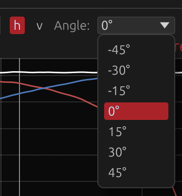
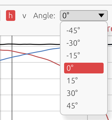
Axis Selection:
- Toggle between h (horizontal) and v (vertical) axis buttons
- Only available when viewing individual drivers or summed system
- Not available in Room Calibration modes
Angle Dropdown:
- Select from available measurement angles
- Only angles with actual measurement data are shown
- 0° always represents the on-axis reference
Interpreting Off-Axis Curves
Compare off-axis to on-axis:
- Smooth transitions across angles = good dispersion control
- Large deviations at certain angles = beaming or nulls
- Crossover region consistency = proper driver integration
What to look for:
- Beaming: Response drops off rapidly at off-axis angles (high-frequency issue)
- Comb filtering: Peaks and dips that vary with angle (driver interference)
- Crossover lobing: Nulls or peaks appearing at specific off-axis angles near crossover frequency
- Baffle diffraction: Ripples that change with angle at mid-to-high frequencies
Example Interpretation:
Good directivity:
- Off-axis curves smoothly roll off at high frequencies
- No sudden dips, peaks or steps through crossover region
- Consistent shape across ±30° angles
Poor directivity:
- Deep nulls appearing at ±20° near crossover frequency
- Off-axis step in frequency response near a crossover frequency, indicating directivity mismatch between drivers
- Dramatic level changes between neighboring angles
- Comb filtering visible at mid frequencies
Directivity Index (DI) Prediction
The Directivity Index (DI) quantifies how directional your speaker is across the frequency spectrum.
What is DI?
Definition:
\[ \text{DI} = 10 \times \log_{10}(Q) \]
where \(Q\) is the directivity factor
\(Q\) is calculated by spherical integration:
\[ Q = \frac{4\pi}{\int_0^{2\pi} \int_0^{\pi} |H(\theta,\phi)|^2 \sin(\theta) , d\theta , d\phi} \]
Interpretation:
- 0 dB = omnidirectional (radiates equally in all directions)
- Higher values = more directional (sound focused forward)
Typical DI Values
0-3 dB: Wide dispersion
- Subwoofers
- Large woofers at low frequencies
- Most speakers below 200 Hz
3-6 dB: Moderate directivity
- Most drivers at mid frequencies
- Typical 2-way speakers at 1-4 kHz
6-12 dB: Controlled directivity
- Waveguides and horns
- Well-designed constant directivity systems
- Ideal for controlled room interaction
12+ dB: Very directional
- Narrow dispersion (potential beaming issues)
- Extreme horns
- May sound disconnected from room in typical listening spaces
How DI Reflects Filtering
The DI curve shows:
- Combined effect of driver placement and crossover filtering
- Interference between drivers creates peaks/dips in the DI
- Crossover slopes affect how quickly directivity changes
- Time-of-flight differences encode driver spacing in the DI pattern
Example DI Behaviors:
Smooth DI transition:
- Gradual increase from 3 dB at 500 Hz to 6 dB at 4 kHz
- Indicates good driver integration through crossover
DI spike at crossover:
- Peak to 8-10 dB at 2.5 kHz, then drops to 6 dB at 3 kHz
- Indicates on-axis summing peak (lobing) at crossover frequency
- Off-axis response likely has nulls
DI dip at crossover:
- Dip to 0 dB at crossover frequency
- Indicates on-axis null (destructive interference)
- May sound better off-axis than on-axis
Using DI for Design
Target smooth DI transition:
- Avoid sudden changes (>3 dB) in DI through crossover region
- Gradual transitions indicate good driver integration
Avoid sudden DI changes:
- Peaks = on-axis lobing (hot spot)
- Dips = on-axis null (cancellation)
- Both indicate poor crossover alignment
Consider desired room interaction:
- Wider DI (3-6 dB) = more room sound (spacious, diffuse)
- Narrower DI (6-12 dB) = less room sound (direct, focused)
- Match DI to listening environment and preference
Match DI to listening environment:
- Near-field (desktop, mixing): Moderate DI acceptable (3-8 dB)
- Far-field (living room, theater): Wider DI preferred (3-6 dB) to engage room
- Treated rooms: Higher DI acceptable (6-10 dB) due to controlled reflections
Listening Window
The Listening Window curve represents the average frequency response over the angular range that matters most for typical listening positions — the region a listener’s ears are likely to be within.
What is the Listening Window?
The Listening Window is defined as the spatial average of all measured frequency responses within ±30° horizontal and ±10° vertical (inclusive). It captures the sound power arriving at listeners seated slightly off-axis, which is more representative of real-world listening conditions than the strict on-axis response alone.
Display Requirements
The Listening Window curve is shown in the Frequency Responses (Drivers) graph when:
- A valid LinFIR license is active
- At least 2 polar measurements fall within the ±30° horizontal / ±10° vertical window
- The Drivers display mode is selected in the graph toolbar
Visual Appearance
| Property | Value |
|---|---|
| Color | Same as the Sum curve (white in dark mode, black in light mode) |
| Line style | Dashed |
| Label | LW |
The dashed style allows the Listening Window and the solid Sum (on-axis) curve to be distinguished at a glance on the same plot.
Interpreting the Listening Window
LW ≈ Sum (on-axis):
- The speaker’s balance changes little within the listening window
- Indicates excellent controlled directivity in the ±30°H / ±10°V region
- High confidence that off-axis listeners experience a similar tonal balance
LW rolls off above Sum at high frequencies:
- Normal and expected behaviour (drivers beam at high frequencies)
- The high-frequency roll-off shape indicates how quickly the speaker narrows
- A gentle, smooth roll-off indicates controlled directivity
LW has dips or irregularities not present on-axis:
- Lobing, comb filtering or directivity discontinuities within the listening window
- May indicate a crossover alignment issue affecting near-axis radiation
- A sudden dip at a specific frequency often points to interference between drivers
Comparing LW with DI:
- As DI rises, the LW typically diverges from the on-axis Sum (more directional → more off-axis loss)
- A flat DI with a flat LW indicates a well-controlled constant-directivity design
Directivity Analysis Window
The Directivity Analysis window displays two complementary visualizations of how sound radiates across frequency and angle. It is organized into two tabs:
- Sonogram — colour-mapped 2D heatmap (frequency × angle)
- Overlay Plot — all off-axis curves superimposed on a single frequency-response graph
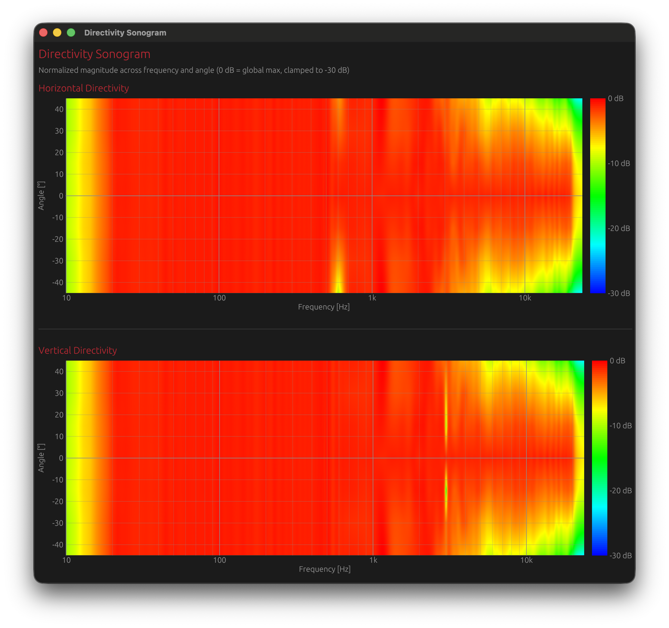
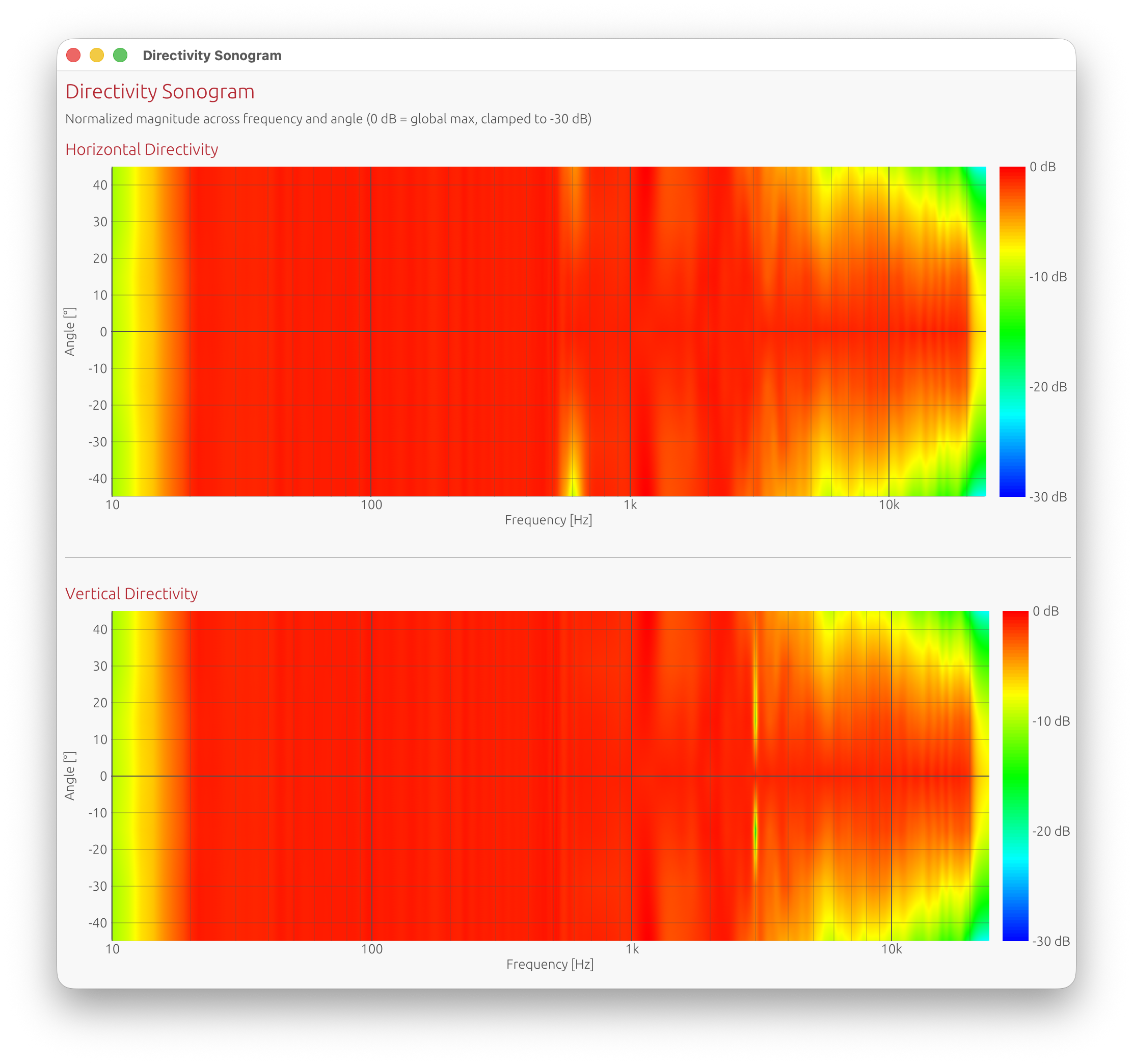
Accessing the Window
Menu: View → Directivity Analysis Requires: Valid LinFIR license and polar measurements loaded
Sonogram Tab — Layout
Two separate sonogram plots:
- Horizontal directivity: Vertical angle = 0°, varying horizontal angle
- Vertical directivity: Horizontal angle = 0°, varying vertical angle
Axes:
- X-axis: Frequency (Hz, logarithmic scale)
- Y-axis: Measurement angle (degrees)
- Color: Normalized magnitude in dB (0 dB = global maximum)
Color Scale
Hot colors (red/yellow): Higher SPL (0 to -6 dB)
- On-axis or near-axis energy
- Focused radiation
Warm colors (orange): Moderate attenuation (-6 to -12 dB)
- Moderate off-axis output
- Typical dispersion
Cool colors (blue/purple): Significant attenuation (-12 to -30 dB)
- Heavily attenuated off-axis
- Beaming or nulls
Range clamped to -30 dB for clarity (adjustable in settings)
Colormap Range Controls
The Colormap range row in the sonogram toolbar lets you saturate the colour scale to reveal low-amplitude detail without reloading any measurement data.
| Control | Description |
|---|---|
| Min dB (drag-value) | Lower saturation threshold — anything at or below this value is rendered in cold blue |
| Max dB (drag-value) | Upper saturation threshold — anything at or above this value is rendered in hot red |
| Reset button | Restores min to the configured magnitude lower bound and max to 0 dB |
How to use it:
- Widen the range (e.g. −60 dB to 0 dB) to get a broad overview of the full dynamic range
- Narrow the range (e.g. −15 dB to −5 dB) to zoom in on mid-level detail and expose subtle lobing or diffraction artefacts that would otherwise blend into a unique color
- Changing either value triggers an immediate image regeneration; the previous image remains visible while the new one is computed
The colorbar on the right of each sonogram always reflects the current min/max values and its grid step adapts automatically to the selected range.
Interpreting Sonograms
Horizontal bands:
- Similar spectral balance across angles
- A band remaining coherent from about −60° to +60° indicates a well-designed driver with controlled directivity and no excessive beaming
Angular width and color spread:
- Warm colors extending from −90° to +90° in the bass / low-midrange are normal (low frequencies are inherently near-omnidirectional)
- Progressive narrowing at high frequencies is expected, but confinement to < −45° to +45° suggests excessive beaming
Symmetry around 0°:
- Geometrical and acoustical symmetry
- Proper driver placement and reliable measurements
Asymmetric patterns:
- Potential baffle diffraction
- Room reflections contaminating measurements
- Driver offset or asymmetric waveguides (intentional in most 3 way monitor designs)
Interference patterns (diagonal/complex):
- Driver interaction visible
- Crossover region summing effects
- Time-of-flight encoding driver spacing
What to Look For
Good Patterns:
Smooth color transitions:
- Gradual change from hot (on-axis) to cool (off-axis)
- Indicates controlled directivity
Symmetric patterns:
- Equal radiation to left/right (horizontal) or up/down (vertical)
- Indicates Symmetric design
Horizontal bands in crossover region:
- Consistent radiation pattern through crossover
- Good driver integration
Bad Patterns:
Narrow bright vertical regions:
- Beaming (concentrated energy on-axis)
- Excessive directivity at that frequency
- Often caused by large drivers at high frequencies
Dark spots off-axis / Diagonal stripes:
- Nulls or cancellations between drivers
- Indicates poor crossover alignment or lobing
- May be acceptable if smooth and symmetric
- Often caused by driver spacing and time-of-flight
- Crossover regions with insufficient acoustic slope, producing off-axis lobing
Crossover Design Insights
Compare on-axis and off-axis patterns:
- Check for consistent summing across all angles
- Look for lobing (bright spots appearing at off-axis angles)
Verify driver summing:
- Crossover frequency should show smooth transition in sonogram
- Moderate nulls or peaks appearing at specific angles
Adjust crossover if needed:
- Lobing visible: Try different crossover slopes or frequency
- Nulls visible: Check driver polarity and time alignment
Example Adjustments:
Problem: Bright and wide lobe at +30° near crossover frequency Solution: Lower crossover frequency or increase slope to reduce overlap
Problem: Null at 0° (on-axis) at crossover frequency Solution: Check driver polarity, adjust time delay, or change crossover type
Problem: Vertical bright bands alternating with dark bands Solution: Driver spacing issue (comb filtering) - may require physical redesign
Overlay Plot Tab
The Overlay Plot tab shows all measured off-axis frequency responses superimposed on a single graph, one coloured line per angle. It complements the sonogram by making it easier to read precise frequency-domain differences between angles.
Horizontal and vertical directivity are displayed one above the other, each with its own set of controls.
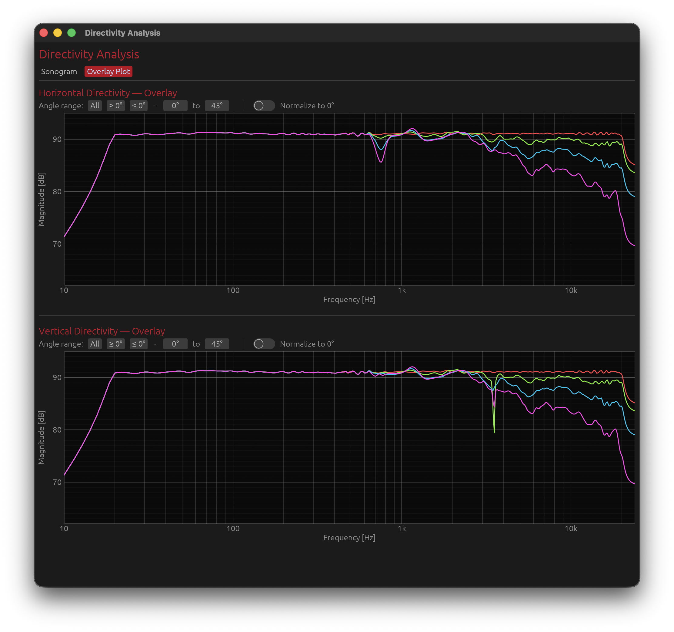
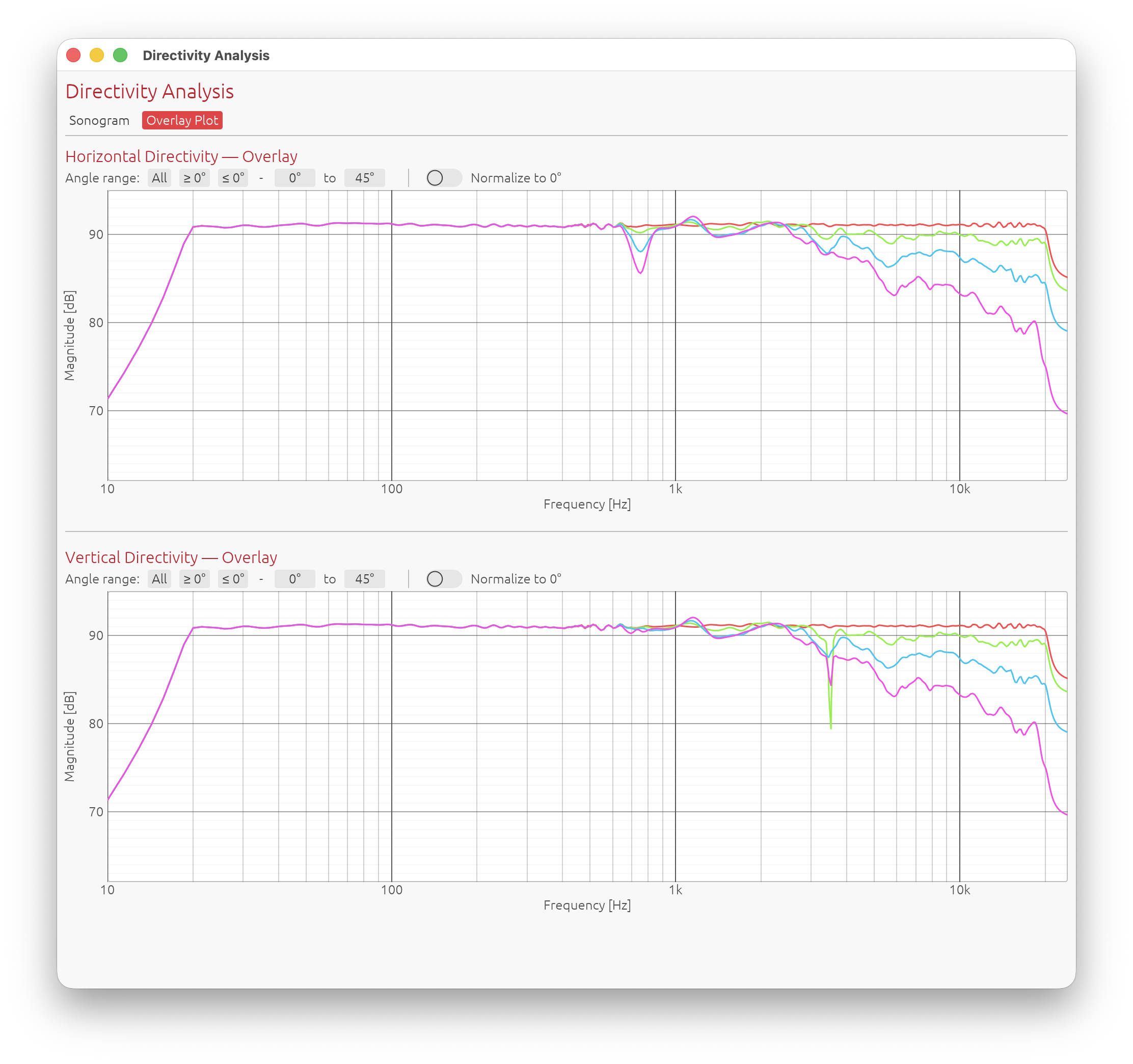
Curve Colours
Angles are mapped to a rainbow colour scale (red → yellow → green → cyan → blue → violet) from the minimum to the maximum angle in the current filter selection.
The angle, frequency, and magnitude are shown in a tooltip when hovering over a curve.
Angle Range Filter
Three preset buttons restrict which angles are plotted:
| Button | Effect |
|---|---|
| All | Show all measured angles |
| ≥ 0° | Positive angles only (0° to max) — default |
| ≤ 0° | Negative angles only (min to 0°) |
A drag-value min/max selector allows fine-grained control of the displayed range. The Y-axis auto-scale updates whenever the selection changes.
Normalize to 0°
The Normalize to 0° toggle divides each curve by the on-axis (0°) response:
- The on-axis curve becomes flat at 0 dB
- All other curves show their deviation relative to on-axis at each frequency
- The Y-axis label changes to Relative Magnitude [dB]
- The vertical range is anchored to the configured magnitude lower bound (e.g. −30 dB to +3 dB)
Interpreting the Overlay Plot
Tightly clustered curves:
- Similar response at all angles → well-controlled directivity
- Especially important in the crossover region
Curves spreading at high frequencies:
- Normal behaviour — drivers beam as frequency rises
- A gradual, smooth spread indicates controlled directivity
Sudden divergence at a specific frequency:
- Possible crossover lobing or driver interference at that frequency
- Cross-reference with the sonogram to confirm
With Normalize to 0° enabled:
- Flat normalized curves (near 0 dB) across ±30° indicate a speaker whose tonal balance is consistent within the listening window
- A normalized curve that drops sharply above a certain frequency indicates the onset of beaming
Why Time-of-Flight Matters
Physics of Multi-Driver Interference
When multiple drivers reproduce the same frequency range, their outputs combine in space. The phase relationship between drivers depends on:
- Physical separation between drivers (geometry)
- Acoustic path length differences to the measurement point
- Crossover filter phase shifts
How Time-of-Flight Encodes This
Each driver’s impulse arrives at a slightly different time:
- This delay represents the acoustic path length to the microphone
- At the on-axis position, path lengths may be similar
- At off-axis positions, path length ratios change
Off-axis measurements capture geometry:
- Driver A might be 1.0 meters away on-axis
- Driver B might be 1.05 meters away on-axis (5 cm path difference)
- At +30° off-axis, Driver A might be 0.95 m and Driver B might be 1.15 m (20 cm difference)
- This changing path length ratio creates interference patterns
These delays create directivity:
- At some frequencies, drivers sum constructively (in phase)
- At other frequencies, drivers sum destructively (out of phase)
- The frequency where this happens depends on the angle (because path lengths change with angle)
- This is the fundamental physics of directivity
What Happens If You Remove TOF without keeping relative delays
Time-aligning removes geometric delay information:
- All drivers appear to arrive at the same time
- DI calculation assumes drivers are co-located (all at the same point in space)
- This is physically incorrect for real speakers
Predicted interference patterns don’t match reality:
- Off-axis nulls and peaks won’t appear
- Directivity sonograms show incorrect lobing
- DI curve does not reflect actual radiation pattern
Example:
With TOF preserved:
- Tweeter and woofer are 15 cm apart vertically
- At 2.3 kHz (wavelength ≈ 15 cm), expect null at certain off-axis angles
- DI curve shows this correctly
With TOF removed (time-aligned):
- Software thinks drivers are co-located
- Predicts no null at 2.3 kHz
- DI curve is smooth (incorrect)
- Real speaker still has null at 2.3 kHz off-axis
Proper Workflow
1. Capture IR with full time-of-flight intact
- Use proper timing reference (electric loopback or acoustic chirp)
- Do not apply windowing that removes acoustic delay
- Preserve the natural arrival time differences
2. Import into LinFIR preserving the delay
- Keep the raw impulse peak positions as captured or remove the same amount of time across all measurements
- Each angle will have slightly different delay values (this is correct)
3. Apply crossover filters
- Crossovers add their own phase shifts
- These combine with geometric delays
4. LinFIR predicts directivity
- Calculation includes both geometry (TOF) and filtering (crossover phase)
- Spherical integration over all measured angles
- Result: realistic DI and sonograms
5. Sonogram shows realistic interference
- Interference patterns reflect both driver spacing and crossover design
- Allows optimization of crossover for desired directivity
Limitations and Best Practices
Measurement Density
More angle measurements = more accurate prediction
- Minimum recommended: 7 angles per axis (±90° in 30° steps)
- Good: 13 angles per axis (±90° in 15° steps)
- Ideal: 19 angles per axis (±90° in 10° steps) or finer
Why density matters:
- DI calculation uses spherical integration
- Sparse measurements = poor integration accuracy
- Fine measurements = more accurate directivity prediction
Room Reflections
Directivity analysis is most accurate in anechoic conditions
- Room reflections distort off-axis measurements
- Early reflections appear as interference in the sonogram
- Can create false lobing patterns
Mitigation strategies:
- Measure outdoors (less reflections)
- Measure in large room with speaker away from walls
- Use gating/windowing carefully:
- Remove late reflections (>10 ms after main arrival)
- Use Adaptive Window to preserve bass while gating reflections
Microphone Position
Keep measurement distance constant:
- Same distance for all angles
- Ensures consistent SPL normalization
- Eliminates distance-related level variations
Farfield measurements (>1 meter) work best:
- Avoids nearfield effects
- Drivers behave as coherent sound sources
- More accurate directivity prediction
Microphone height:
- Should match speaker acoustic center
- For 2-way speaker, typically between tweeter and woofer
- Ensures symmetric vertical measurements
Computational Notes
DI calculation uses spherical integration:
- Computationally intensive (integrates over all angles and frequencies)
- May take a few seconds for dense polar data
Sonogram generation:
- Creates high-resolution 2D images (frequency × angle)
- Parallel processing used for speed
- Results are cached to improve performance
Getting a License
To unlock Directivity Analysis tools:
- Visit the LinFIR website: https://linfir.demaudio.com
- Purchase a license key
- Enter your e-mail and key in LinFIR: Settings → License
- All directivity features will be enabled immediately
Your license supports:
- Ongoing development
- New features
- Bug fixes and improvements
Related Documentation
- IR Management: Capturing and managing off-axis measurements
- Audio Setup: Configuring audio interface, measurement settings, and timing reference for accurate polar measurements
- Driver Processing: Crossover design and optimization
Summary
Directivity Analysis tools characterize how your speaker radiates sound in different directions:
Features:
- Off-axis frequency response visualization at any angle
- Directivity Index (DI) prediction across the spectrum
- Directivity sonograms (2D colour-mapped heatmaps, frequency × angle)
- Overlay Plot (all off-axis curves superimposed, with angle range filter and normalize to 0° toggle)
Requirements:
- Valid LinFIR license
- Polar measurements at multiple angles (horizontal and vertical)
- Preserved time-of-flight
- Proper timing reference (electric loopback or acoustic chirp)
Key Concepts:
- Time-of-flight encodes driver geometry (must be preserved)
- DI quantifies how directional the speaker is (0 dB = omni, higher = more directional)
- Sonograms visualize radiation patterns (hot colors = on-axis energy, cool = off-axis attenuation)
- Overlay Plot superimposes all off-axis curves for precise frequency-domain comparison; normalize to 0° shows deviation relative to on-axis
- Crossover optimization based on directivity for consistent off-axis response
Workflow:
- Configure timing reference (electric loopback recommended)
- Capture polar measurements for each drivers (preserve time-of-flight)
- Design crossovers and apply filters
- View off-axis curves, DI, sonograms, and overlay plots
- Optimize crossover for desired directivity pattern
- Iterate based on measurements
Use directivity analysis to understand and optimize your speaker’s radiation pattern for better room interaction and consistent sound across the listening area.
Distortion Impulse Responses 🔒
License Required: The Distortion IR window requires a valid LinFIR license.
The Distortion IR window visualises the time-domain harmonic impulse responses (\(h_2\) through \(h_5\)) extracted from an ESS (Exponential Sine Sweep) Farina measurement. It shows the same windowed slices used to compute the THD spectrum.
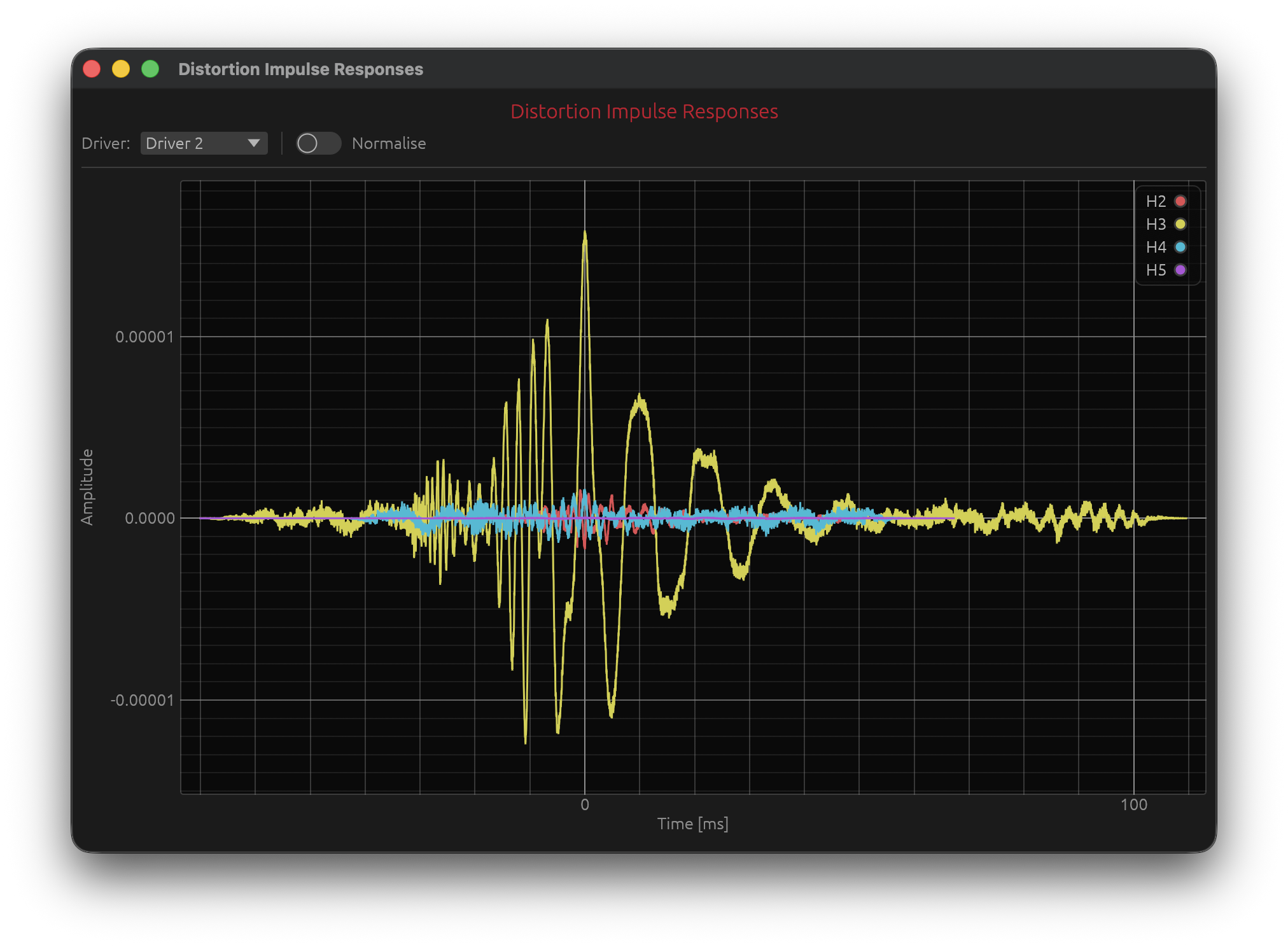
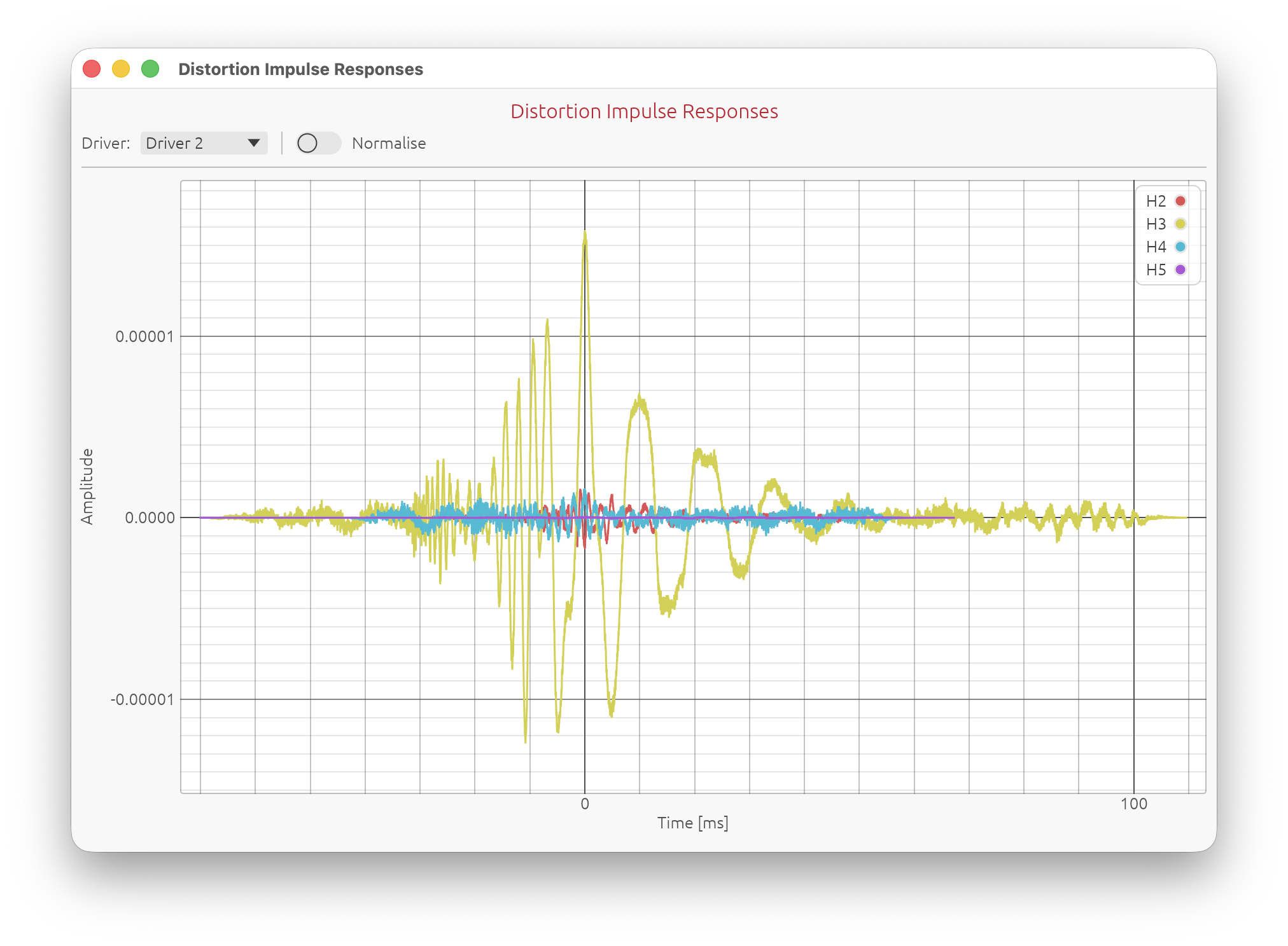
Accessing the Distortion IR Window
Menu: View → Distortion IR
Keyboard shortcut: J
The window is available in Loudspeaker Design and Hypex FusionAmp modes, and requires that at least one driver has a valid ESS harmonic measurement.
What It Shows
When a driver is measured using the Sweep Measurements system (ESS method), LinFIR separates the harmonic components of the impulse response using the Farina deconvolution technique. Each harmonic order (k) arrives at a distinct, predictable time offset before the fundamental:
$$\Delta t_k = \frac{T_s \cdot \ln(k)}{\ln(f_2 / f_1)}$$
where \(f_1\), \(f_2\) are the sweep start and end frequencies and \(T_s\) the sweep duration.
The Distortion IR window displays these separated impulse response slices — \(h_2\), \(h_3\), \(h_4\), \(h_5\) — on a shared time axis, with all peaks aligned to the same time origin so the shape of each harmonic can be compared directly.
Angle Dependence
The displayed measurement follows the global angle selector. When a non-zero horizontal or vertical angle is selected, the window shows the harmonic impulse responses from the matching off-axis measurement (if one exists). The window title and header update to indicate the active angle, e.g.:
Distortion Impulse Responses — +15°H +0°V
If no measurement exists for the selected angle, the window automatically falls back to the on-axis (0°H 0°V) measurement.
Controls
Driver Selector
A ComboBox at the top of the control bar selects which driver’s harmonic slices are displayed.
Normalise
The Normalise toggle scales each harmonic curve independently so its peak amplitude equals 1.0. This makes the shape of each impulse response directly comparable regardless of the absolute distortion level.
With normalisation disabled, the amplitudes are proportional to the actual distortion levels.
Note: Normalise is a purely visual operation. It does not affect the underlying computation or the THD/distortion values in the main graphs.
Extraction and Windowing
Each harmonic slice is extracted as follows:
- Theoretical peak positions for \(h_2\)–\(h_{MAX}\) are computed from the ESS parameters.
- Cut points are located at the minimum of the smoothed Hilbert envelope between each pair of adjacent theoretical peaks, with a 5 % margin on each side to avoid touching either peak. This maximises the separation between harmonics and adapts automatically to any sweep duration or sample rate.
- Each slice is extracted between its two cut points — no overlap between adjacent harmonics.
- Sub-sample fractional delay correction is applied to align each harmonic to its exact theoretical position.
- Phase offset correction removes the constant phase bias introduced by the Farina deconvolution for each harmonic order.
- DC removal is applied.
- A 5 % raised-cosine fade-in / fade-out is applied to both ends of the slice before peak alignment. This windowing is independent for each harmonic and does not depend on the \(h_1\) IR window settings, because harmonic impulse responses can extend significantly further in time than the fundamental.
- All slices are zero-padded at the front so their peaks are aligned to a common time reference.
Distortion IR window shows the slices exactly as they enter the THD spectrum computation.
Requirements
- Driver must have an ESS sweep capture (exponential sine sweep measurement via Sweep Measurements).
- A valid LinFIR license is required to open the window.
Related Documentation
- Sweep Measurements — ESS measurement procedure and parameters
- Driver Processing — IR windowing for the fundamental \(h_1\)
- Spectrogram — time-frequency view of the full impulse response
- Directivity Analysis — off-axis frequency response visualisation
- License — license features and activation
Export & Project Management
This section covers exporting filters, total impulse responses, and managing your LinFIR projects.
Filter Export
Overview
LinFIR allows you to export processed FIR filter coefficients for use in external DSP systems, hardware amplifiers, or room correction software. You can export:
- Individual Driver FIR Filters: Per-driver crossover and correction filters (Loudspeaker Design mode only)
- Global FIR Correction: System-wide magnitude and phase correction filters
- Total Impulse Response: The complete processed system impulse at the listening position
Access: Menu > Export Filters
Important: Driver Adjustments Are Not Exported
⚠️ Critical Note: Filter exports (FIR and IIR) do NOT include Driver Adjustments (gain, time delay, and polarity inversion).
What’s Exported:
- FIR filter coefficients (crossovers + correction)
- IIR filter coefficients (parametric EQ, shelving, etc.)
What’s NOT Exported:
- 🔊 Gain adjustment (-40 to +40 dB)
- ⏱️ Time delay (0 to 100 ms)
- 🔄 Polarity inversion (180° phase flip)
Why?
These parameters are intentionally excluded for both technical and practical reasons.
Gain Embedding a gain offset directly into FIR coefficients (scaling all taps) seems harmless, but can silently cause internal clipping in some DSP architectures — particularly fixed-point or integer pipelines where the headroom available after the FIR stage is limited. DSP platforms provide dedicated gain controls for precisely this reason: they operate at the right stage in the signal chain and respect the hardware’s dynamic range constraints.
Time delay
Baking a time delay into a FIR filter is a costly misuse of resources. It works by translating the filter impulse response within its tap window: the filter is shifted right by N samples, zeros are prepended on the left, and the same number of meaningful taps are truncated on the right. This has two consequences:
- Filter truncation introduces artefacts — the discarded taps carry real filter information (typically the ringing or low-frequency content of the impulse). Losing them degrades the filter’s frequency and phase response.
- Convolving zeros is wasteful — a DSP has to compute multiplications on those leading zeros at every sample, consuming CPU cycles or DSP MAC operations to produce nothing. By contrast, every DSP platform offers dedicated delay lines (circular buffers, integer sample delay blocks) that implement delay at essentially zero computational cost. They are the right tool for the job.
Polarity inversion A simple sign flip on all coefficients works mathematically, but like gain, it is directly available as a single-bit inversion in every DSP, with no processing overhead.
In short: each of these adjustments has a dedicated, efficient, and precise implementation in your DSP. Keeping them separate from the FIR data gives you full control and avoids hard-to-debug artefacts.
What You Must Do: After exporting filters, you must manually configure these parameters in your target DSP:
- Set each driver’s output gain/level
- Configure time delay/alignment for each channel
- Enable polarity inversion where needed
Exception:
- Hypex HFD Export (→ see HFD Export section): Gain, delay, and polarity are automatically included in the
.hfdconfiguration file
Export File Formats
LinFIR supports multiple export formats to ensure compatibility with various DSP platforms:
Binary Formats
- FLOAT32LE (
.bin): IEEE 754 32-bit little endian float- Standard format for CamillaDSP and MiniDSP
- Raw binary data, no header
- Each sample is 4 bytes
- FLOAT64LE (
.bin): IEEE 754 64-bit little endian float- Higher precision for demanding applications
- Raw binary data, no header
- Each sample is 8 bytes
Text Formats
- CSV row (
.csv): Comma-separated values in a single row - CSV column (
.csv): One coefficient per line - Text decimal (
.txt): Decimal format, one coefficient per line:0.123456 - Text scientific (
.txt): Scientific notation format, one coefficient per line:1.2345600000000000e-01
Audio Formats
- WAV 16-bit (mono) (
.wav): 16-bit integer PCM- Auto-normalized: Coefficients are automatically normalized to prevent clipping if max(abs(value)) > 1.0
- Range: -32768 to 32767 (maps to -1.0 to 1.0)
- Single channel audio file
- WAV 24-bit (mono) (
.wav): 24-bit integer PCM- Auto-normalized: Coefficients are automatically normalized to prevent clipping if max(abs(value)) > 1.0
- Range: -8388608 to 8388607 (maps to -1.0 to 1.0)
- Single channel audio file
- WAV 32-bit float (mono) (
.wav): 32-bit floating point- Raw coefficients: No normalization, values preserved as-is (can exceed ±1.0)
- Same data as FLOAT32LE binary format, but with WAV header
- Single channel audio file
- WAV 16-bit (stereo) (
.wav): 16-bit integer PCM stereo- Auto-normalized: Coefficients are automatically normalized to prevent clipping if max(abs(value)) > 1.0
- Range: -32768 to 32767 (maps to -1.0 to 1.0)
- Dual channel audio file with identical left/right channels (mono signal duplicated)
- WAV 24-bit (stereo) (
.wav): 24-bit integer PCM stereo- Auto-normalized: Coefficients are automatically normalized to prevent clipping if max(abs(value)) > 1.0
- Range: -8388608 to 8388607 (maps to -1.0 to 1.0)
- Dual channel audio file with identical left/right channels (mono signal duplicated)
- WAV 32-bit float (stereo) (
.wav): 32-bit floating point stereo- Raw coefficients: No normalization, values preserved as-is (can exceed ±1.0)
- Dual channel audio file with identical left/right channels (mono signal duplicated)
Note on Normalization: FIR filter coefficients can have values outside the ±1.0 range. WAV PCM formats (16-bit, 24-bit) automatically normalize coefficients to fit their limited integer range while preserving the filter’s frequency response shape. WAV 32-bit float and binary formats (FLOAT32LE/FLOAT64LE) preserve raw coefficient values without normalization.
Note on Stereo Formats: Stereo WAV formats duplicate the mono FIR filter signal to both left and right channels. The actual filter data is identical in both channels.
Platform-Specific Formats
- Text - Powersoft Armonia (
.txt): Format for Powersoft amplifiers. Usually requires 48 kHz to be set as target sampling frequency.
FIR Export Process
When exporting FIR filters (Menu > Export Filters):
- Driver Selection: In Loudspeaker Design mode, LinFIR exports each enabled driver with active FIR filters (HP, LP, or correction)
- Only enabled drivers are exported (drivers with the Enabled button toggled on in the Drivers toolbar)
- Disabled drivers are automatically skipped during export
- Global Filter: If global FIR correction is enabled, it’s exported as a separate file
- Room Calibration Mode: Only global filters are exported (no per-driver files)
- File Naming: Each filter gets a descriptive name with complete parameter details by default
Filter Naming Convention
Exported filter names include all relevant parameters for complete traceability:
Driver FIR Example:
Tweeter_4096taps_96000Hz_HPLR4-2500Hz_CORR(MAG+PH_R30dB_G-2.5dB_MinPhase).wav
Components:
Tweeter: Driver name (from imported IR filename)4096taps: Filter length (including padding)96000Hz: Sample rateHPLR4-2500Hz: High-pass Linkwitz-Riley 4th-order at 2500 Hz- Format:
HPorLP+ filter type abbreviation + order (if not brick-wall) +-+ frequency - Types: Brick-wall (no order),
BW(Butterworth),LR(Linkwitz-Riley),BE(Bessel)
- Format:
CORR(...): Correction filter details (only if correction is enabled)MAG+PH: Both magnitude and phase correction enabledMAGorPH: Only one correction type enabledR30dB: 30 dB correction range (magnitude only)G-2.5dB: -2.5 dB post-gain (magnitude only, only if gain ≠ 0)MinPhase: Minimum-phase causality (causality ≥ 0.99)C75%: Mixed causality at 75% (causality 0.01-0.98)- No causality suffix = Linear-phase (causality = 0.0)
Global FIR Example:
GlobalFIR_8192taps_96000Hz_MAG_R40dB_C50%_200-18000Hz.wav
Components:
GlobalFIR: Global correction identifier8192taps: Filter length (including padding)96000Hz: Sample rateMAGorPHorMAG+PH: Correction type enabledR40dB: 40 dB correction range (magnitude only)G+2.5dB: Post-gain in dB (only if gain ≠ 0)MinPhase: Minimum-phase (causality ≥ 0.99)C50%: Mixed causality at 50% (0.01-0.98)- No causality suffix = Linear-phase (causality = 0.0)
200-18000Hz: Frequency range (only if f_min > 20 Hz or f_max < Nyquist - 100 Hz)
Padding and Filter Length
Exported filters include:
- Base taps: The configured filter length (N taps)
- Padding taps: Additional zero-padding if configured
Padding ensures compatibility with DSP systems that require a specific fixed tap count (e.g., Hypex amplifiers and DSPs require specific lengths).
Room Calibration Export Behavior
In Room Calibration mode:
- Only global filters are exported (no per-driver FIR files)
- The global FIR represents the averaged correction across all measurement positions
- Individual driver controls are disabled in this mode
- Export focuses on the overall room response correction
IIR Filter Export
Overview
LinFIR can export IIR filters (digital biquad coefficients) in four formats:
- FQG Format (
.txt): Text-based frequency/Q/gain lists - CamillaDSP Format (
.yml): YAML configuration for CamillaDSP - Q-SYS Format (
.csv): CSV biquad coefficients for Q-SYS IIR Custom Filter - MiniDSP Format (
.txt): Compact biquad coefficients for MiniDSP devices
Note: Only IIR filters from enabled drivers are exported. Disabled drivers are automatically skipped.
IIR export is available for:
- Global IIR filters (system-wide EQ and crossovers)
- Per-driver IIR filters (individual driver EQ, in Loudspeaker Design mode)
Export Formats
FQG Format (Text)
Simple text format listing filter parameters:
# Global IIR Filters (FQG Format)
# Sample Rate: 96000 Hz
# Format: Type [Pass] Frequency [Order] [Q] [Gain]

Butterworth HP 80.0 4
Butterworth LP 20000.0 4
PEQ 1200.0 2.500 -3.50
LowShelf 200.0 0.707 2.00
HighShelf 10000.0 0.707 -1.50
Allpass2 3000.0 1.414
Allpass1 500.0
Format Details:
- Butterworth/LR/Bessel:
Type Pass Frequency Order- Pass:
HP(high-pass) orLP(low-pass)
- Pass:
- PEQ:
PEQ Frequency Q Gain - Low/High Shelf:
LowShelf/HighShelf Frequency Q Gain - Allpass2:
Allpass2 Frequency Q(second-order) - Allpass1:
Allpass1 Frequency(first-order)
CamillaDSP Format (YAML)
Full YAML configuration with native CamillaDSP filter types:
# Global IIR Filters (CamillaDSP Format)
# Sample Rate: 96000 Hz
filters:

  filter_1:
    type: BiquadCombo
    parameters:
      type: ButterworthHighpass
      freq: 80.0
      order: 4

  filter_2:
    type: Biquad
    parameters:
      type: Peaking
      freq: 1200.0
      gain: -3.50
      q: 2.500

  filter_3:
    type: Biquad
    parameters:
      type: Lowshelf
      freq: 200.0
      gain: 2.00
      q: 0.707
CamillaDSP Native Types:
ButterworthLowpass/ButterworthHighpassLinkwitzRileyLowpass/LinkwitzRileyHighpassPeaking(PEQ)Lowshelf/HighshelfAllpass(second-order)AllpassFO(first-order)
Bessel Filters: CamillaDSP doesn’t natively support Bessel filters, so they’re exported as Free biquad sections with explicitly calculated coefficients:
  filter_1_1_bessel:
    type: Biquad
    parameters:
      type: Free
      b0: 0.9876543210123456
      b1: -1.9753086420246912
      b2: 0.9876543210123456
      a1: -1.9750000000000000
      a2: 0.9755086580370370
Q-SYS Format (CSV)
CSV format for Q-SYS IIR Custom Filter components. Each line represents one biquad section with coefficients in the order: b0, b1, b2, a0, a1, a2.
0.0040888760000000, 0.0081777519000000, 0.0040888760000000, 1.0000000000000000, -1.8954199260000000, 0.9117754299000000,
0.0040888760000000, 0.0081777519000000, 0.0040888760000000, 1.0000000000000000, -1.8954199260000000, 0.9117754299000000,
0.0033894348000000, 0.0067788696000000, 0.0033894348000000, 1.0000000000000000, -1.7990948390000000, 0.8126525782000000,
Format Specification:
- One biquad section per line
- Coefficients:
b0, b1, b2, a0, a1, a2,(trailing comma optional) - Coefficient
a0must be non-zero (normalized to 1.0 by LinFIR) - 16 decimal places precision for maximum accuracy
- Compatible with Q-SYS Designer IIR Custom Filter component
Usage in Q-SYS:
- Export filters from LinFIR in Q-SYS format
- In Q-SYS Designer, add an IIR Custom Filter component
- Set the component’s Section Count property to match the number of lines in your CSV file
- Close and reopen the component’s control panel
- Load the CSV file using the Coefficient File property
Important Notes:
- Each filter in LinFIR may generate multiple biquad sections (see Biquad Count Reference below)
- High-order filters (e.g., Butterworth 8th order) will create multiple CSV lines
- Total biquad count = sum of all lines in the CSV file
MiniDSP Format (Text)
Compact text format with biquad coefficients for MiniDSP hardware processors. Each biquad section is labeled and coefficients are provided in normalized form.
biquad1,
b0=0.9876543210123456
b1=-1.9753086420246912
b2=0.9876543210123456
a1=-1.9750000000000000
a2=0.9755086580370370
biquad2,
b0=1.0123456789012345
b1=-2.0246913578024690
b2=1.0123456789012345
a1=-1.9980000000000000
a2=0.9960493580246914
Format Specification:
- Each biquad section starts with
biquadN,where N is the section number (1, 2, 3, …) - Coefficients are listed one per line in the order:
b0,b1,b2,a1,a2 - Note:
a0is omitted (assumed to be 1.0 after normalization) - Format:
coefficient_name=valuewith no spaces around the=sign - 16 decimal places precision for maximum accuracy
Important Notes:
- Each filter in LinFIR may generate multiple biquad sections (see Biquad Count Reference below)
- MiniDSP devices have limited biquad slots
- High-order filters will consume multiple biquad slots
- Check your device’s specifications for maximum biquad count before exporting complex filter chains
Biquad Count Reference
Understanding biquad counts is essential when exporting to hardware with limited DSP resources (e.g., Hypex FA series amplifiers with a 15-biquad limit):
| Filter Type | Order | Biquad Count |
|---|---|---|
| Butterworth/Bessel LP/HP | 1 | 1 |
| Butterworth/Bessel LP/HP | 2 | 1 |
| Butterworth/Bessel LP/HP | 3 | 2 |
| Butterworth/Bessel LP/HP | 4 | 2 |
| Butterworth/Bessel LP/HP | 5 | 3 |
| Butterworth/Bessel LP/HP | 6 | 3 |
| Butterworth/Bessel LP/HP | 7 | 4 |
| Butterworth/Bessel LP/HP | 8 | 4 |
| Butterworth/Bessel LP/HP | 9 | 5 |
| Butterworth/Bessel LP/HP | 10 | 5 |
| Linkwitz-Riley LP/HP | 2 (LR2) | 2 |
| Linkwitz-Riley LP/HP | 4 (LR4) | 2 |
| Linkwitz-Riley LP/HP | 8 (LR8) | 4 |
| Linkwitz-Riley LP/HP | 10 (LR10) | 5 |
| PEQ (Parametric EQ) | - | 1 |
| Low/High Shelf | - | 1 |
| Allpass2 (2nd-order) | - | 1 |
| Allpass1 (1st-order) | - | 1 |
Linkwitz-Riley Formula: LR filters are implemented as cascaded Butterworth sections:
- LR order = 2 × Butterworth order
- LR2 = 2× Butterworth 1st-order = 2 biquads
- LR4 = 2× Butterworth 2nd-order = 2 biquads
- LR8 = 2× Butterworth 4th-order = 4 biquads
Butterworth/Bessel Formula: Biquad count = ⌈order / 2⌉ (ceiling of order divided by 2)
Export Process
- Open Menu > Export IIR Filters
- Select export format (FQG, CamillaDSP, Q-SYS, or MiniDSP)
- LinFIR identifies all enabled IIR filter chains:
- Global IIR (if enabled)
- Per-driver IIR (if enabled, Loudspeaker Design mode only)
- For each filter chain, specify output filename
- Files are generated with complete filter specifications
Room Calibration Mode: Only global IIR filters are exported (no per-driver files).
HFD Export (Hypex FA Series)
Overview
LinFIR can generate Config.xml project files for Hypex FA series amplifiers:
- FA251, FA501 (1-channel with DSP)
- FA122, FA252, FA502 (2-channel with DSP)
- FA123, FA253, FA503 (3-channel with DSP)
About
Config.xml: This is the native project file format used by the Hypex Filter Design (HFD) software. HFD opens and uploadsConfig.xmlfiles directly to FA series amplifiers. LinFIR generates a ready-to-useConfig.xmlthat you can open in HFD immediately.
This integration enables direct deployment of your loudspeaker designs to Hypex amplifiers without manual coefficient transfer.
✅ Driver Adjustments Included: Unlike standard FIR/IIR exports, HFD export automatically includes gain, time delay, and polarity settings for each driver. These are written directly into the
Config.xmlfile and applied by the amplifier.
Supported Device Models
| Model | Channels | Max FIR (Input) | Max FIR (Output/ch) | Max IIR (biquads/ch) |
|---|---|---|---|---|
| FA122 | 2 | 4500 taps | 1500 taps | 15 |
| FA123 | 3 | 4500 taps | 1500 taps | 15 |
| FA251 | 1 | 4500 taps | 1500 taps | 15 |
| FA252 | 2 | 4500 taps | 1500 taps | 15 |
| FA253 | 3 | 4500 taps | 1500 taps | 15 |
| FA501 | 1 | 4500 taps | 1500 taps | 15 |
| FA502 | 2 | 4500 taps | 1500 taps | 15 |
| FA503 | 3 | 4500 taps | 1500 taps | 15 |
Requirements
Sample Rate: HFD export requires 93.75 kHz sample rate
- FA series amplifiers operate at 93.75 kHz internally
- If your LinFIR project uses a different sample rate, you must change it before HFD export
- Set Sampling Frequency to 93.75 kHz in Target DSP Settings
Biquad Limit: Maximum 15 biquads per channel
- LinFIR automatically counts biquads when exporting
- Global IIR filters + driver IIR filters must not exceed 15 biquads per output channel
- See Biquad Count Reference for calculation details
FIR Position: Choose between two FIR filter placement options:
-
Input FIR (Global, 4500 taps maximum):
- Single FIR filter applied to the input signal before channel routing
- Suitable for global room correction or full-range equalization
- More efficient for shared corrections across all channels
-
Output FIR (Per-channel, 1500 taps maximum per channel):
- Independent FIR filters for each output channel
- Suitable for per-driver crossover and correction filters
Export Workflow
1. Configure HFD Settings
Open Menu > Export HFD to access the HFD export window:
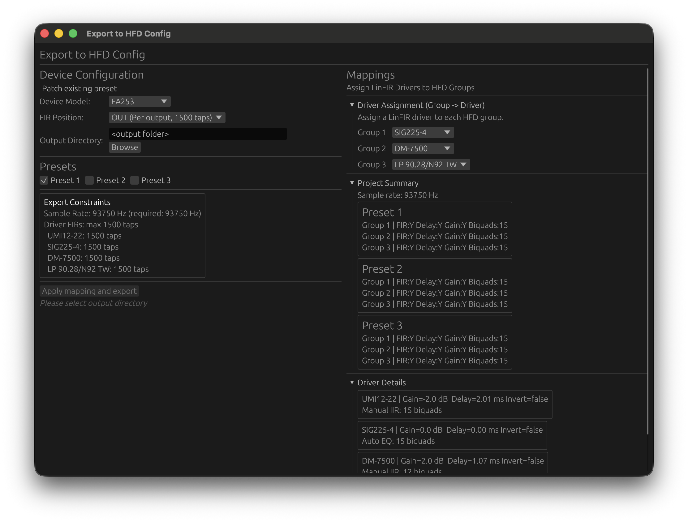

- Mode: Choose between Create from template or Patch existing Config.xml (see Patch Mode)
- Device Model: Select your Hypex FA amplifier model
- FIR Position: Choose Input (global) or Output (per-channel) FIR placement
- Channel-to-Driver Mapping: Assign the filters of each LinFIR driver to a FusionAmp output channel
2. Map Drivers to FusionAmp Channels
The mapping table assigns the FIR filters, IIR filters, gain, delay, and polarity computed for each LinFIR driver to a specific FusionAmp output channel. Channels are numbered as they appear in the HFD Config.xml.
By default, LinFIR assigns drivers sequentially: the first driver goes to Channel 1, the second to Channel 2, and so on. If there are fewer drivers than channels, the last driver is repeated for the remaining channels.
| FusionAmp Channel | LinFIR Driver | Notes |
|---|---|---|
| Channel 1 | Driver 1 (Woofer) | Output channel 1 |
| Channel 2 | Driver 2 (Mid) | Output channel 2 |
| Channel 3 | Driver 3 (Tweeter) | Output channel 3 |
Mapping Validation:
- LinFIR checks that all mappings are valid before export
- Warnings appear if biquad count exceeds 15 for any channel
- FIR length validation ensures compliance with Input (4500) or Output (1500) tap limits
3. Select Presets to Export
Hypex FA amplifiers support multiple configuration presets (typically 3). Choose which presets to include in the exported HFD file:
- ☑ Preset 1: Main tuning
- ☑ Preset 2: Alternate voicing
- ☐ Preset 3: (Skip)
Uncheck presets you don’t want to modify in the existing configuration.
4. Patch Mode (Update Existing Configuration)
Patch Mode allows you to update an existing Config.xml instead of creating one from scratch. Select Patch existing Config.xml in the Mode dropdown.
- Select Mode: Set the Mode dropdown to Patch existing Config.xml
- Browse: Click Browse… and select the
Config.xmlfile on your disk - LinFIR will:
- Auto-detect the FIR position (Input or Output) from the loaded file
- Parse existing presets and channel configurations
- Lock FIR position and device model to match the loaded file
- Update Selected Presets: Only the presets you’ve checked will be modified; others remain unchanged
- Click Apply mapping and export — the selected
Config.xmlis overwritten in place
Use Cases for Patch Mode:
- Update filter coefficients after design refinements
- Safely modify one preset without affecting others
- Create different presets (boosted bass, different voicing, etc.)
5. Validation and Export
Before exporting, LinFIR performs comprehensive validation:
Biquad Count Check:
Tweeter has 18 biquads but HFD supports max 15 biquads per channel
Reduce IIR or Auto-EQ filter count for this driver.
FIR Length Check - Position Input:
Global FIR has 6000 taps but Input position supports max 4500 taps
Reduce global FIR length or switch to Output position.
FIR Length Check - Position Output:
Woofer has 2000 taps but Output position supports max 1500 taps per channel
Reduce driver tap count or switch to Input position.
Sample Rate Check:
HFD export requires 93.75 kHz sampling rate. Current: 96000 Hz
Change sample rate to 93.75 kHz in Settings.
If validation passes, click Apply mapping and export:
- In Create from template mode: a Save As dialog opens — choose the location and filename (
Config.xmlis pre-filled) - In Patch mode: the selected
Config.xmlis overwritten in place immediately
A confirmation message is shown below the export button on success.
6. Load Configuration to Amplifier
Use Hypex Filter Design (HFD) to upload the exported Config.xml to your FA series amplifier:
- Connect amplifier via USB
- Open Hypex Filter Design (HFD)
- Open the exported
Config.xmlfile (File > Open Project) - Click Upload to Device
Total Impulse Response Export
Overview
Export the complete processed impulse response at the listening position (acoustic sum of all enabled drivers + global filters).
This is useful for:
- External room correction systems (e.g., Audiolense, Acourate, etc.)
- Validation and measurement (import into REW, Matlab, etc.)
- Archival and comparison (document before/after tuning)
Export Options
Menu > Export Predicted Total IR (TXT/WAV)
WAV Export
- Format: 32-bit float WAV (single channel)
- Sample Rate: Choose target sample rate (can differ from project sample rate)
- LinFIR will resample automatically if needed
- Common rates: 44.1 kHz, 48 kHz, 96 kHz, 192 kHz
Example: Export at 48 kHz for compatibility with external room correction software, even if your project is at 96 kHz.
TXT Export
- Format: Plain text, one sample per line (decimal)
- Sample Rate: Choose target sample rate (with automatic resampling)
- Use Cases: Import into Matlab, Python (numpy), or custom DSP tools
Resampling Behavior
If the target sample rate differs from your project sample rate:
- LinFIR uses high-quality resampling (sinc interpolation)
- The exported impulse maintains accurate time-domain characteristics
- No manual resampling required
Example Workflow:
- LinFIR project at 96 kHz (high precision for design)
- Export total impulse at 48 kHz (target hardware sample rate)
- LinFIR handles resampling transparently
Project Management
Saving Projects
LinFIR projects are saved as .lnf files containing:
- Driver configurations (impulse responses, filters, gain, delay, polarity)
- Global FIR and IIR filter settings
- Display preferences and graph states
- Project mode (Loudspeaker Design or Room Calibration)
- Measurement data (including off-axis measurements)
Save Shortcut: Cmd+S (macOS) / Ctrl+S (Windows/Linux)
Save Options
- Menu File/Save (or Cmd+S): Overwrites the current project file
- Menu File/Export/LinFIR Project: Creates a new project file with a specified name
- Auto-Save: Enabled by default
- Automatically saves every 60 seconds if changes detected
- Runs in background without blocking the UI
Loading Projects
Menu > File/Load Project
LinFIR supports:
- New format (
.lnf): Current project structure with full multi-angle measurement support - Legacy format: Older LinFIR project files (automatically migrated on load)
Legacy Migration: When loading an old project file:
- LinFIR converts the structure to the new format
- A notification confirms successful migration
- Re-save the project to preserve the new format
Drag & Drop
Drag .lnf files directly onto the LinFIR window to open projects.
Unsaved Changes Protection:
- If you have unsaved changes, LinFIR prompts:
You have unsaved changes. Save before opening?
[Save] [Don't Save] [Cancel]
Recent Projects
Access recently opened projects from Menu > Recent Projects:
- Up to 20 recent projects listed
- Click to open instantly
- List persists across sessions
Related Documentation
- Driver Processing - FIR crossovers and correction filters
- System Processing - Global FIR and IIR filters
- Keyboard Shortcuts - Complete shortcut reference
Troubleshooting
This guide covers common issues and their solutions when using LinFIR.
Sweep Measurement Issues
Capture Rejected - Clipping Detected
Error Message: Capture rejected: Clipping detected! Reduce input gain and try again.
Cause: The recorded signal exceeded 0 dBFS (digital full scale), causing clipping/distortion.
Solutions:
- Reduce input gain on your audio interface
- Lower driver volume or move microphone further away from the speaker
- Check gain staging throughout the signal chain:
- Audio interface preamp gain
- Mixer/console levels (if used)
- Microphone sensitivity
- Verify microphone input isn’t overloading (check interface clip indicators)
- Use pad/attenuation if your microphone or interface has this option
Prevention: Start with low input gain and gradually increase while monitoring level meters during test sweeps.
Capture Rejected - Signal Too Low
Error Message: Capture rejected: Signal too low (-XX.X dB)! Increase input gain and try again.
Cause: The recorded signal is below -25 dBFS, resulting in poor signal-to-noise ratio.
Solutions:
- Increase input gain on your audio interface
- Raise driver volume or move microphone closer to the speaker
- Check microphone connection:
- Ensure cable is properly connected
- Verify phantom power is enabled (for condenser microphones)
- Test microphone with other software to confirm it’s working
- Verify audio routing:
- Confirm correct input channel is selected in Audio Settings
- Check that no mute or pad switches are engaged
- Ensure audio interface is set as the active input device
Target Level: Aim for peak levels between -12 dBFS and -6 dBFS for optimal signal-to-noise ratio.
Timing Reference Issues
Error Message: Timing reference not detected (correlation too low: -XX.X dB). Check channels and levels.
Cause: LinFIR cannot detect the timing reference signal (Acoustic or Loopback mode).
Solutions:
For Acoustic Timing Reference:
- Verify microphone positioning: Timing reference speaker must be within the microphone’s field
- Check timing reference level: Signal should be audible
- Increase output level of the timing reference channel
- Verify channel routing: Ensure timing reference is sent to the correct output
For Loopback Timing Reference:
- Verify physical loopback cable is properly connected
- Check loopback input channel selection in Audio Settings
- Ensure loopback signal isn’t attenuated (no pads, no gain reduction)
- Test loopback path independently (send signal and monitor input)
Error Message: Timing reference signal is CLIPPING (≥ 0 dBFS). Reduce timing reference output level or input gain to prevent distortion.
Solution: Reduce output level or input gain for the timing reference channel until clipping stops.
No Audio During Sweep
Symptoms: Sweep doesn’t play, or plays but no sound is heard.
Solutions:
- Verify device selection in Audio Settings tab:
- Output device is correct
- Input device is correct
- Channels are properly mapped
- Check hardware connections:
- Audio interface is powered on
- Speakers/amplifiers are connected and powered
- Cables are properly seated
- System audio settings:
- Ensure audio interface is not muted in system settings
- Check exclusive mode settings (Windows)
- Verify sample rate compatibility
- Try different buffer sizes:
- Start with 512 or 1024 samples
- Increase if experiencing dropouts
- Test with another application to confirm audio interface is functioning
Windows Specific: Disable exclusive mode for the audio device in Windows Sound Settings if LinFIR cannot access it.
Poor Quality Measurements
Symptoms: Noisy frequency response, irregular impulse response, inconsistent results.
Solutions:
- Use longer sweep duration:
- Minimum 5 seconds for small rooms
- 10+ seconds for large rooms or outdoor measurements
- Longer sweeps improve signal-to-noise ratio
- Minimize background noise:
- Turn off HVAC systems during measurement
- Close windows and doors
- Avoid traffic noise or other environmental sounds
- Choose quiet times of day
- Ensure stable microphone positioning:
- Use a sturdy microphone stand
- Avoid vibrations from speakers at high SPL
- Mark microphone position for repeatability
- Check for electrical interference:
- Use balanced cables (XLR) where possible
- Avoid running audio cables parallel to power cables
- Check for ground loops (hum at 50/60 Hz and harmonics)
- Use isolated/clean power for sensitive equipment
- Use multiple averages:
- 3-5 averages reduce random noise
- More averages improve consistency at the cost of time
- Verify measurement environment:
- Avoid highly reflective surfaces near microphone
- Ensure speaker is properly positioned
- Check for loose objects that might rattle
Unstable Audio Scheduling (Windows)
Error Message: Recording rejected: unstable Windows audio scheduling.
Cause: Windows audio subsystem experienced excessive timing jitter during capture.
Solutions:
- Close other applications using audio or consuming CPU
- Increase buffer size in Audio Settings (try 1024 or 2048 samples)
- Disable audio enhancements in Windows Sound Settings
- Update audio interface drivers to latest version
- Use ASIO drivers if available for your interface (more stable than WASAPI)
- Disable background services:
- Windows Update
- Antivirus real-time scanning
- Other system services during measurement
- Check power settings: Set to “High Performance” mode
IR Management Issues
File Import Problems
Symptoms: Cannot import WAV or TXT files, or imported data appears incorrect.
Solutions:
WAV Files:
- Verify file format: Only WAV files are supported (16/24/32-bit PCM or float)
- Check file integrity: Ensure file isn’t corrupted or truncated
- Try opening in another audio application
- Re-export from source if needed
- Sample rate must be reasonable: 44.1 kHz to 192 kHz
- Stereo files: LinFIR uses left channel only (mono conversion)
- Check file permissions: Ensure LinFIR has read access to the file
TXT (IR) Files:
- Format must be simple: One sample per line, decimal values
- Sample rate prompt: LinFIR will ask for sample rate (not stored in TXT)
- Check for non-numeric characters: Remove headers, comments, or invalid data
- Use proper decimal separator: Period (
.) not comma (,)
FRD (.frd or .txt) Files (REW format):
- Two-column format: Frequency (Hz) and Magnitude (dB)
- Tab or space delimited
- Check frequency range: Should cover at least 20 Hz to 20 kHz
- Phase column: Optional third column for phase (degrees)
Windowing Not Working
Symptoms: IR windowing doesn’t change the impulse response, or produces unexpected results.
Solutions:
- Verify time values:
- Stop Time must be > Start Time
- Times must be within IR duration
- Window times are in milliseconds, not samples
- Preview impulse response to verify window placement:
- Open Driver IR window
- Check impulse response plot
- Adjust Start/Stop times visually
- Common windowing scenarios:
- Early reflections removal: Set Stop Time before first strong reflection
- Noise truncation: Set Stop Time when IR decays into noise floor
- Leading silence removal: Set Start Time just before main impulse peak
IR Names Not Showing
Symptoms: Imported or measured impulse responses don’t have names, or show default names.
Explanation: LinFIR does not automatically set IR names based on filenames or measurements.
Solutions:
- Manually enter IR name:
- Open Driver IR window
- Type name in “IR Name” field
- Press Enter or click outside field to confirm
- Import and measurement operations:
- WAV import: No automatic naming
- Sweep measurement: No automatic naming
- FRD import: No automatic naming
- Save project to persist custom names:
- Use Cmd+S / Ctrl+S to save
- IR names are stored in project file
Best Practice: Name impulses immediately after import/measurement to avoid confusion later.
Audio Settings Issues
Device Not Listed
Symptoms: Expected audio interface doesn’t appear in device dropdown menus.
Solutions:
- Click “Refresh Devices” to rescan audio hardware
- Check audio interface:
- Ensure interface is powered on
- Verify USB/Thunderbolt connection is secure
- Try different USB port or cable
- Verify drivers are installed:
- Mac OS: Core Audio drivers (usually automatic)
- Windows: ASIO or manufacturer-specific drivers
- Close other applications using the audio interface:
- DAWs (Pro Tools, Logic, Ableton, etc.)
- Media players
- Communication apps (Zoom, Microsoft Teams, etc.)
- Try different sample rates or buffer sizes in LinFIR settings
- Restart LinFIR after connecting/disconnecting devices
- System permissions (Mac OS):
- Go to System Settings > Privacy & Security > Microphone
- Ensure LinFIR has microphone access
Configuration Invalid
Error: Audio configuration shows as invalid or cannot be applied.
Causes and Solutions:
-
Device disconnected:
- Selected input/output device is no longer available
- Click “Refresh Devices” and reselect devices
-
Channel count exceeds device capabilities:
- Verify device has enough input/output channels
- Check channel mapping (e.g., selecting channel 8 on a 2-channel interface)
-
Sample rate not supported:
- Audio interface may not support selected sample rate
- Try common rates: 48 kHz, 96 kHz, 44.1 kHz
- Check interface specifications
-
Buffer size incompatible:
- Some devices have minimum/maximum buffer size limits
- Try 512 or 1024 samples as a safe default
-
Exclusive mode conflicts (Windows):
- Another application may have exclusive control
- Disable exclusive mode in Windows Sound Settings
- Close competing applications
Recovery Steps:
- Click “Refresh Devices”
- Select “Default” input and output devices
- Choose a common sample rate (48 kHz)
- Set buffer size to 1024 samples
Filter Processing Issues
FIR Correction Not Applying
Symptoms: Enabling FIR correction doesn’t change frequency response.
Solutions:
- Check correction is enabled:
- Magnitude and/or Phase correction must be toggled ON
- Verify correction range (Max. Attenuation) is non-zero (e.g., 10 dB)
- Check frequency range covers desired bandwidth
- Verify target curve:
- Check that your reference points are defined correctly
- Reference shouldn’t be identical to measurement (no correction needed)
- Check causality setting:
- Linear phase (causality = 0): Maximum pre-ringing
- Minimum phase (causality = 1): No pre-ringing, phase distortion
- Mixed causality (0 < causality < 1): Balanced trade-off
- Increase filter length if correction is insufficient:
- Longer FIR = better correction accuracy
- Try doubling N taps (e.g., 2048 → 4096)
- View FIR filter response in Filters mode (F key):
- Switch to display mode “FIR Filters”
- Verify correction filter shape matches expectation
- Check FIR time alignment:
- Verify that the FIR coefficients are properly centered within the available taps
- Try changing FIR Offset Delay value to recenter FIR’s energy
- Enable Auto Causal Alignment in Settings and let LinFIR handle this process for you
Cannot See IIR Filter Effects
Symptoms: IIR filters are defined but don’t affect the frequency response.
Causes and Solutions:
-
IIR toggle is disabled:
- Click the “IIR Filters” toggle in the driver toolbar to enable it
- Both Manual IIR and Auto-EQ tabs share this same master toggle
-
Wrong tab is active:
- LinFIR has two separate IIR filter tabs: Manual and Auto-EQ
- Only the active tab’s filters are applied
- Click the tab you want to use to make it active
- You can have filters in both tabs, but only one tab is active at a time
-
No filters are enabled:
- In the active tab, verify that individual filters have their “Enabled” toggle ON
- Disabled filters are ignored even if the tab is active
-
Switching between Manual and Auto-EQ:
- Manual IIR tab: Manually configured filters (HP, LP, PEQ, shelves, etc.)
- Auto-EQ tab: Auto-generated or manually tweaked parametric EQ filters
- Use “Clone from Auto EQ” button to copy Auto-EQ filters to Manual tab
- Both tabs can coexist with different filter sets, but only one is active
Auto-EQ Not Matching Target
Symptoms: Auto-EQ result doesn’t match target curve well.
Solutions:
- Increase max filters allowed:
- More filters = better target matching
- Try 8-12 filters for complex targets
- Check frequency range:
- Auto-EQ only operates within specified f_min to f_max
- Reduce range if needed (e.g., 80 Hz to 16 kHz)
- Verify target curve is reasonable:
- Avoid extreme target shapes requiring >20 dB boost
- Use smooth target curves for better results
- Check smoothing:
- Over-smoothed measurements may prevent accurate matching
- Try 1/12 or 1/24 octave smoothing
- Run Auto-EQ again:
- Click “Run Auto EQ” to recompute
- Different starting conditions may produce better results
HFD Export Issues
Sample Rate Error
Error: HFD export requires 93.75 kHz sampling rate. Current: 96000 Hz
Solution: Hypex FA series amplifiers operate at 93.75 kHz internally.
Steps:
- Go to Target DSP Settings in the left column of the main window
- Change Sampling Frequency to 93.75 kHz
- Retry HFD export
Note: Changing sample rate will trigger re-processing of all filters.
Biquad Limit Exceeded
Error: Tweeter has 18 biquads but HFD supports max 15 biquads per channel
Cause: The sum of global IIR + driver IIR exceeds 15 biquads per output channel.
Solutions:
- Reduce IIR filter count:
- Remove unnecessary PEQ filters
- Combine shelves into broader adjustments
- Use fewer global IIR filters
- Reduce Auto-EQ filter count:
- Lower “Max Filters” setting in Auto-EQ
- Simplify target curve to require fewer filters
- Move filters to FIR domain:
- FIR crossovers instead of IIR (if tap budget allows)
- FIR correction instead of many PEQ filters
- Check biquad count for each filter type (see table in Export documentation)
Example:
- Driver IIR: LR4 HP, LR4 LP, 12× PEQ
- Total: 16 biquads ❌ Exceeds limit
Solution: Reduce PEQs to 11 filters → Total: 15 biquads ✅
FIR Length Exceeded
Error:
Global FIR has 6000 taps but Input position supports max 4500 tapsWoofer has 2000 taps but Output position supports max 1500 taps per channel
Cause: FIR filter length exceeds Hypex hardware limits.
Solutions:
For Input FIR (Global, 4500 taps max):
- Reduce Global FIR N taps in Global FIR Correction settings
For Output FIR (Per-channel, 1500 taps max):
- Reduce Driver N taps in driver settings
Decision Guide:
- Input FIR: Best for global room correction shared across all channels
- Output FIR: Best for per-driver crossovers and correction
Performance Issues
Slow Processing / UI Lag
Symptoms: LinFIR feels sluggish, filters take long to compute, UI updates are delayed.
Solutions:
- Reduce filter complexity:
- Lower FIR tap count (e.g., 4096 → 2048)
- Fewer IIR filters
- Disable unused filters
- Reduce graph resolution:
- Settings > Graphs > Plot Resolution
- Lower resolution = faster rendering
- Disable unnecessary graphs:
- Hide graphs you’re not using (M, P, G, I, T, K keys)
- Fewer visible graphs = less computation
- Close detached graph windows when not needed
- Check system resources:
- Close other CPU-intensive applications
- Ensure sufficient RAM available
- Reduce angle step in polar measurements:
- Try 10° or 15° steps instead of 5°
High Memory Usage
Symptoms: LinFIR consumes excessive RAM, system becomes slow.
Causes:
- Many drivers with long IRs: Each driver stores full impulse responses
- Many polar measurements: Full impulse responses are also stored for each measurement angle
- High-resolution graphs: More points = more memory
Solutions:
- Reduce IR length re-import externally generated IRs with proper windowing and truncation
- Use lower sample rates if 192 kHz is not needed
- Reduce N taps for FIR filters
- Reduce graph resolution Settings > Graphs > Plot Resolution
Project File Issues
Cannot Load Project
Error: Failed to load project or similar error when opening .lnf file.
Solutions:
- Check file integrity:
- Verify file size is reasonable (not 0 bytes)
- Legacy format migration:
- Older LinFIR versions may use incompatible format
- LinFIR attempts automatic migration, but may fail
- Try opening in latest LinFIR version
- Corrupted project:
- If file was saved during a crash, it may be incomplete
- Restore from a backup
- File permissions:
- Ensure LinFIR has read access to the file
- Try copying file to a different location
Prevention: Enable auto-save to save every 60 seconds.
Auto-Save Not Working
Symptoms: Projects don’t auto-save, or auto-save notifications don’t appear.
Verification:
- Auto-save is enabled by default
- Auto-save runs every 60 seconds in the background
- Auto-save only works if project has a saved path (use Cmd+S first time)
Troubleshooting:
- Save project manually first (Cmd+S) to establish a file path
- Check for errors: Look for error notifications in top-right corner
- Verify file permissions: Ensure LinFIR can write to project directory
- Check disk space: Ensure sufficient free space on drive
Note: Auto-save interval cannot be configured (fixed at 60 seconds).
License & Activation Issues
Directivity Features Locked
Symptoms: Cannot access the directivity analysis window (R key doesn’t work), directivity features grayed out.
Cause: Directivity analysis requires a valid license.
Solutions:
- Verify license status: Settings > License tab
- Activate license: Enter license key if you have one
- Check license expiration: Licenses may have time limits (trial)
- Mode requirement: Directivity is only available in Loudspeaker Design mode (not Room Calibration)
- Check internet connectivity: First activation (or deactivation) requires internet connectivity
Note: Free version includes all core loudspeaker design features but excludes advanced directivity analysis.
Getting Help
Bug Reports
LinFIR includes a built-in bug report feature to help diagnose issues:

To Submit a Bug Report:
- Go to Help > Report a Bug
- Describe the issue clearly:
- What you were doing when the problem occurred
- What you expected to happen
- What actually happened
- Include steps to reproduce (if possible)
- Click “Submit”
Privacy:
- No personal information is transmitted
- No project data is included
- Only relevant log information and system details are sent
What to Include:
- Clear description of the bug or unexpected behavior
- Exact steps to reproduce the issue
- Expected vs. actual outcome
- System information: OS version, audio interface model (if relevant)
- Error messages (if any appear)
Community & Support
Additional Resources:
- User Manual: Press H to open embedded documentation
- Release Notes: Check for known issues and recent fixes
- Email Support: Contact developer for persistent issues
Before Reporting:
- Check this troubleshooting guide
- Verify you’re using the latest LinFIR version
- Test with a fresh project to isolate the issue
- Try restarting LinFIR and your audio interface
Related Documentation
- Audio Configuration - Detailed audio settings and device configuration
- Sweep Measurements - Measurement procedures and best practices
- IR Management - Importing, windowing, and managing impulse responses
- Export & Project Management - HFD export requirements and validation
- Keyboard Shortcuts - Quick reference for all shortcuts
Acoustic Advisory
This section provides important guidance on the physical limitations of DSP-based room correction and loudspeaker design.
The Limits of DSP Correction
Understanding Physical Nulls
Deep cancellations (nulls) from room modes or driver boundary interference (SBIR - Speaker Boundary Interference Response) are physical destructive interference patterns and generally cannot be “fixed” by boosting with FIR correction or IIR PEQ.
Why Nulls Cannot Be Corrected:
- Destructive Interference: Nulls occur when direct sound and reflected sound arrive out of phase, canceling each other
- Spatial Dependency: The cancellation exists at specific locations but not everywhere in the room
- Energy Conservation: You cannot add energy where none exists due to phase cancellation
- Headroom Waste: Boosting into nulls consumes massive headroom without improving the actual acoustic situation
Example: A 20 dB null at 80 Hz cannot be filled by adding 20 dB boost at 80 Hz. The boost will:
- Waste amplifier power
- Increase distortion
- Worsen the response at other listening positions
- Create excessive excursion demands on drivers
EQ Best Practices
What EQ Can Fix
Effective Uses of EQ:
- Broad, minimum-phase peaks: Driver resonances, baffle diffraction effects
- Overall target shaping: House curve, tilt, broad spectral balance
- Crossover integration: Blending drivers at crossover region
- Driver mismatch correction: Sensitivity differences between drivers
Example: A 5 dB broad peak at 3 kHz from a tweeter resonance is an ideal candidate for PEQ correction.
What EQ Cannot Fix
Ineffective Uses of EQ:
- Deep, narrow nulls (> 6-8 dB depth): Room modes, SBIR, comb filtering
- Path length cancellation: Nulls from multiple drivers or reflections
- Non-minimum-phase dips: Cannot be corrected without introducing pre-ringing
- Spatial nulls: Cancellations that vary significantly with listener position
Example: A 15 dB null at 50 Hz from a room mode should be addressed with:
- Subwoofer repositioning
- Multiple subwoofers (spatial averaging)
- Bass traps and acoustic treatment
- Listener position adjustment
Not with: A 15 dB PEQ boost at 50 Hz
Boost Guidelines
Conservative Boost Limits
General Recommendations:
- Avoid large boost into deep nulls: Limit boost to ~6-8 dB maximum
- Focus on peaks, not nulls: Cutting peaks is acoustically sound, boosting nulls is not
- Relatively broad adjustments: Wide Q filters (0.5-6.0) for gentle shaping
- Preserve headroom: Every dB of boost reduces available headroom
Why 6-8 dB Limit?:
- Beyond this level, you’re likely boosting into a physical null
- Distortion increases exponentially with excursion (especially at low frequencies)
- Power requirements increase by 2× per 3 dB boost
- Thermal compression reduces actual output gain
Boost vs. Cut Philosophy
Prefer Cutting over Boosting:
- Cut peaks: Removes excess energy without headroom penalty
- Boost sparingly: Only for broad, gentle shaping
- Net gain reduction: Apply global gain to compensate for cuts
Example Workflow:
- Identify a broad peak at 2 kHz (+4 dB)
- Cut with PEQ: -4 dB at 2 kHz, Q = 1.0
Room Correction Strategies
Spatial Averaging (Multiple Mic Positions)
Why Multiple Positions Matter:
- Room modes and nulls vary significantly with position
- Single-point measurements can be misleading
- Averaging reduces emphasis on position-specific anomalies
- Produces more robust correction that works across a larger listening area
Recommended Approach:
- Measure at 3-5 positions within the listening area
- Use Room Calibration mode in LinFIR to average responses
- Apply correction based on averaged response
- Focus on fixing common peaks across all positions
- Ignore position-specific nulls (cannot be fixed for all positions)
Physical Solutions First
Order of Priority:
-
Speaker and Listener Placement:
- Wall distance: Keep speakers 5 cm to 1 m from rear wall
- Avoid placing directly against walls (especially with rear-ported designs)
- Don’t exceed ~1 m distance to prevent comb filtering issues in bass/low-midrange
- Closer placement (<50 cm) shifts SBIR null higher in frequency (less problematic with speaker directivity)
- Farther placement (50-100 cm) shifts SBIR null lower in frequency (more problematic for bass)
- Adjust listening position to avoid room mode nulls
- Use the “rule of thirds” as a base for room placement
- Experiment with toe-in and speaker spacing
- Wall distance: Keep speakers 5 cm to 1 m from rear wall
-
Bass Management:
- Multiple subwoofers for spatial averaging
- Distributed Bass Array (DBA) for modal smoothing
- Subwoofer crawl technique to find optimal placement
- Phase and time alignment between subs and mains
-
Acoustic Treatment:
- Bass traps in corners for low-frequency modal control
- Absorption at first reflection points
- Diffusion on rear wall for controlled reflections
-
DSP Correction (Last Step):
- Correct broad, minimum-phase peaks
- Apply target curve shaping
- Light smoothing of overall response
- Do not aggressively boost nulls
Frequency Region Strategies
Below Room Transition (Schroeder Frequency)
Characteristics:
- Strong modal behavior (room modes dominate)
- Deep nulls and sharp peaks
- Response varies dramatically with position
- Typically 80-200 Hz depending on room size
Recommended Approach:
- Repositioning and treatment are most effective
- Use multiple subwoofers for spatial averaging
- Apply bass traps to control modal ringing
- Light EQ for broad peaks only (avoid boosting nulls)
- Expect imperfect results (physics limits DSP)
Why EQ Struggles:
- Nulls are spatial (different at every position)
- Boosting nulls creates problems at other positions
- Time-domain ringing (long decay times) cannot be fixed with EQ
Above Room Transition Frequency
Characteristics:
- Direct sound dominates
- Room modes are no longer the primary issue
- Speaker-room interaction remains important (perceived sound = direct + reflections)
- Two design philosophies emerge:
- Wide directivity: Uses room reflections for spaciousness (requires good crossover design)
- Controlled directivity: Limits room interaction for consistency across spaces
- Typically 200-300 Hz and above
Recommended Approach:
- Gate/window measurements to emphasize direct sound
- Focus on crossover design and driver integration
- EQ for target curve shaping and driver correction
- Time-align drivers for proper summation
Measurement Technique:
- Use impulse response windowing to exclude reflections
- Set window to capture direct sound only (e.g., 5-10 ms after arrival)
- This removes room influence and focuses on loudspeaker design
Speaker Boundary Interference Response (SBIR)
What is SBIR?
SBIR occurs when direct sound from a speaker combines with its reflection from a nearby boundary (floor, wall, ceiling).
Characteristics:
- Deep null at \(f_{null} = \frac{c}{4d}\) where \(c\) = speed of sound (343 m/s), \(d\) = distance to boundary
- Example: Speaker 1 meter from wall → null at ~86 Hz
- Cannot be fixed with EQ (phase cancellation)
Solutions:
- Move speaker closer to boundary: Drecreases \(d\), shifts null to higher frequency (less problematic with speaker directivity)
- Subwoofer integration: Crossover below SBIR null frequency
- Accept and avoid: Don’t boost the null, work around it
Why EQ Doesn’t Work:
- Null is caused by phase cancellation (180° out of phase)
- Adding energy (boost) cannot fix phase relationship
- Boosting wastes headroom and creates distortion
LinFIR Design Intent
Primary Use Case: Loudspeaker Design
LinFIR is optimized for:
- Driver and crossover design using anechoic or quasi-anechoic data
- Windowed measurements to isolate direct sound
- Crossover filter design (HP, LP, correction)
- Driver integration and phase alignment
- Target curve shaping
Best Results With:
- Outdoor measurements (no room reflections)
- Anechoic chamber measurements
- Gated far-field measurements (remove reflections)
Secondary Use Case: Room Correction
LinFIR can be used for room correction with realistic expectations:
Appropriate:
- Broad spectral balancing (house curve, tilt)
- Correction of broad peaks from room modes
- Light smoothing of overall response
- Spatial averaging across multiple measurement positions
Inappropriate:
- Aggressive boosting of deep nulls
- Single-point correction without spatial averaging
- Expecting perfect flat response in a typical room
- Relying solely on DSP instead of acoustic treatment
Realistic Expectations:
- DSP has fundamental limits
- Room acoustics require multi-faceted approach (placement + treatment + modest EQ)
- Perfect correction is impossible in modal region
- Best results come from combining all techniques
Common Mistakes to Avoid
1. Boosting Nulls Aggressively
Mistake: Applying 15 dB boost to fill a room mode null at 80 Hz.
Why It’s Wrong:
- Null is caused by destructive interference (cannot add energy where none exists)
- Boost increases distortion and thermal compression
- Worsens response at other listening positions
- Wastes amplifier headroom
Correct Approach:
- Reposition subwoofer or listening position
- Add second subwoofer for spatial averaging
- Use bass traps to dampen modal ringing
- Accept a small null (better than aggressive boost)
2. Single-Point Measurement for Room Correction
Mistake: Measuring at one position and correcting for that spot only.
Why It’s Wrong:
- Room response varies dramatically with position (especially below 200 Hz)
- Correction optimized for one spot often worsens others
- Modal nulls and peaks are position-dependent
Correct Approach:
- Measure at 3-5 positions within listening area
- Use Room Calibration mode for spatial averaging
- Correct only features common across all positions
- Ignore position-specific nulls
3. Ignoring Physical Solutions
Mistake: Relying only on DSP to fix all acoustic problems.
Why It’s Wrong:
- Physical placement and treatment are more effective for many issues
- DSP cannot fix phase cancellation, time-domain ringing, or spatial nulls
- Some problems have no DSP solution
Correct Approach:
- Optimize speaker and listener placement first
- Add acoustic treatment (bass traps, absorption, diffusion)
- Use multiple subwoofers if needed
- Apply DSP as final polish (not primary solution)
4. Over-Damping the Room
Mistake: Covering all walls with absorption to eliminate reflections.
Why It’s Wrong:
- Rooms need some reflections for spaciousness and envelopment
- Over-damping creates a “dead” sound
- Low frequencies are unaffected (absorption ineffective below 200 Hz without massive thickness)
Correct Approach:
- Treat first reflection points only
- Use bass traps in corners for low-frequency control
- Add diffusion (not just absorption) for controlled reflections
- Preserve room liveliness (some reflections are good)
5. Excessive FIR Correction Gain
Mistake: Applying FIR correction with 15 dB boost at low frequencies to “flatten” response.
Why It’s Wrong:
- FIR correction amplifies everything, including distortion and noise
- Massive boost wastes headroom
- Likely boosting into nulls that cannot be fixed
- Thermal compression reduces actual gain achieved
Correct Approach:
- Limit FIR correction to reasonable ranges (±6-8 dB)
- Focus on correcting broad peaks (cutting, not boosting)
Summary: Best Practices
DO:
✅ Focus EQ on broad, minimum-phase peaks
✅ Use spatial averaging (multiple mic positions) for room correction
✅ Combine placement, treatment, and modest DSP
✅ Window measurements above transition frequency to isolate direct sound
✅ Limit boost to ~6-8 dB maximum
✅ Prefer cutting peaks over boosting nulls
✅ Use LinFIR for driver and crossover design (primary use case)
DON’T:
❌ Boost deep, narrow nulls (> 6-8 dB)
❌ Rely solely on DSP for room correction
❌ Expect perfect flat response in modal region
❌ Apply single-point correction without spatial averaging
❌ Ignore physical solutions (placement, treatment)
❌ Over-damp the room (preserve some reflections)
❌ Boost nulls caused by SBIR or room modes
Physical Acoustics Primer
Speed of Sound
\(c = 343 \text{ m/s}\) (at 20°C, sea level)
Wavelength Formula: \(\lambda = \frac{c}{f}\)
Examples:
- 20 Hz → 17.15 m wavelength
- 100 Hz → 3.43 m wavelength
- 1 kHz → 0.343 m (34.3 cm)
- 10 kHz → 0.034 m (3.4 cm)
Implications:
- Low frequencies have long wavelengths → difficult to control with treatment
- High frequencies have short wavelengths → easy to absorb, control
Room Modes
Axial Mode Formula (between parallel walls):
\[f_n = \frac{nc}{2L}\]
where \(n\) = 1, 2, 3… (mode number), \(L\) = room dimension
Example (5m room length):
- 1st mode: \(f_1 = \frac{343}{2 \times 5} = 34.3 \text{ Hz}\)
- 2nd mode: \(f_2 = \frac{2 \times 343}{2 \times 5} = 68.6 \text{ Hz}\)
- 3rd mode: \(f_3 = \frac{3 \times 343}{2 \times 5} = 102.9 \text{ Hz}\)
Modal Density: Number of modes per Hz increases with frequency. At high frequencies, modes overlap (modal smoothing).
Schroeder Frequency (Room Transition)
Approximate Formula:
\[f_s \approx 2000 \sqrt{\frac{RT_{60}}{V}}\]
where \(RT_{60}\) = reverberation time (seconds), \(V\) = room volume (m³)
Typical Living Room (50 m³, RT60 = 0.4s):
\[f_s \approx 2000 \sqrt{\frac{0.4}{50}} \approx 179 \text{ Hz}\]
Below \(f_s\): Modal behavior dominates (discrete modes, deep nulls/peaks)
Above \(f_s\): Statistical behavior (modal overlap, smoother response)
Related Documentation
- Room Calibration - Multi-position measurement workflow
- Sweep Measurements - Measurement techniques and best practices
- IR Management - Windowing impulse responses to isolate direct sound
- System Processing - Global FIR correction parameters and limits
- Troubleshooting - Common measurement and processing issues