Directivity Analysis 🔒
License Required: Directivity analysis features require a valid LinFIR license. All other LinFIR features remain free to use.
Directivity analysis tools characterize how your speaker system radiates sound in different directions. These tools predict off-axis behavior, visualize interference patterns between drivers, and help optimize crossover design for consistent directivity.
Overview
Directivity analysis provides:
- Off-axis frequency response visualization at any measured angle
- Directivity Index (DI) prediction across the frequency spectrum
- Directivity sonograms (2D frequency vs. angle heatmaps)
- Crossover optimization insights based on radiation patterns
Key Applications:
- Identify directivity errors, beaming and dispersion characteristics
- Optimize crossover design for consistent off-axis response
- Assess room interaction based on directivity patterns
- Visualize interference patterns between drivers
Polar Measurements
Measurement Requirements
To use directivity tools, you need impulse responses at multiple angles:
Horizontal Axis:
- Measurements with vertical angle = 0°, varying horizontal angle
- Example: -90°, -60°, -30°, 0°, +30°, +60°, +90°
- More angles provide better accuracy (5° or 10° increments recommended)
Vertical Axis:
- Measurements with horizontal angle = 0°, varying vertical angle
- Example: -60°, -40°, -20°, 0°, +20°, +40°, +60°
- Particularly important for speakers with vertical array configurations
On-axis Reference:
- The (0°, 0°) measurement is the on-axis reference
- Must be captured first before off-axis measurements
- Appears in both horizontal and vertical columns in the IR Management window
⚠️ Critical: Time of Flight Must Be Preserved
DO NOT:
- Apply windowing that removes the acoustic delay
- Time-align measurements to the same start point
- Remove the relative delay between drivers
WHY:
- The relative delay between angles encodes interference patterns
- This delay represents the acoustic path length to the microphone
- Off-axis measurements have different path length ratios between drivers
- These delays create the directivity patterns we analyze
What happens if you remove time-of-flight:
- DI calculation assumes drivers are co-located (incorrect)
- Predicted interference patterns don’t match reality
- Off-axis nulls and peaks won’t appear
- Directivity sonograms show incorrect lobing patterns
⚠️ Critical: Use Proper Timing Reference
Configure a timing reference method in Audio Settings before capturing polar measurements:
Electric (loopback) - RECOMMENDED:
- Most reliable method
- Connect output to input with a cable
- Eliminates software scheduler variability
- See Reference Timing for setup
Acoustic (chirp):
- Uses another driver as timing reference microphone
- Good for setups where loopback is impractical
- Requires careful positioning
Avoid “None” timing mode:
- Relies on system audio scheduler (unreliable on Windows)
- Timing jitter corrupts phase relationships between drivers
- Can produce incorrect directivity analysis
💡 Tip: Stable timing is essential for accurate phase relationships between drivers. See Reference Timing for detailed setup instructions.
Measurement Tips
General Guidelines:
- Keep microphone-to-speaker distance constant for all angles
- Rotate the speaker (not the microphone) when possible
- Ensure consistent room conditions for all measurements
- Use high SNR settings to capture clean off-axis data
Distance Recommendations:
- Farfield measurements (>1 meter) work best
- Distance should be at least 2-3× the largest driver spacing
- Too close = nearfield effects, inaccurate directivity
- Too far = room reflections dominate
Microphone Positioning:
- Ensure microphone height matches speaker acoustic center
- Keep microphone axis perpendicular to speaker front baffle
- Avoid obstructions in the measurement path
Off-Axis Curve Visualization
View off-axis frequency responses directly in the main graph window.
Accessing Off-Axis Display
Location: Main graph toolbar (Drivers/Speakers display mode only)
Axis Selection:
- Toggle between h (horizontal) and v (vertical) axis buttons
- Only available when viewing individual drivers or summed system
- Not available in Room Calibration modes
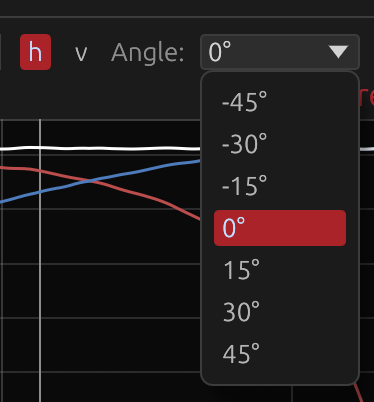
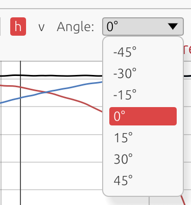
Angle Dropdown:
- Select from available measurement angles
- Only angles with actual measurement data are shown
- 0° always represents the on-axis reference
Interpreting Off-Axis Curves
Compare off-axis to on-axis:
- Smooth transitions across angles = good dispersion control
- Large deviations at certain angles = beaming or nulls
- Crossover region consistency = proper driver integration
What to look for:
- Beaming: Response drops off rapidly at off-axis angles (high-frequency issue)
- Comb filtering: Peaks and dips that vary with angle (driver interference)
- Crossover lobing: Nulls or peaks appearing at specific off-axis angles near crossover frequency
- Baffle diffraction: Ripples that change with angle at mid-to-high frequencies
Example Interpretation:
Good directivity:
- Off-axis curves smoothly roll off at high frequencies
- No sudden dips, peaks or steps through crossover region
- Consistent shape across ±30° angles
Poor directivity:
- Deep nulls appearing at ±20° near crossover frequency
- Off-axis step in frequency response near a crossover frequency, indicating directivity mismatch between drivers
- Dramatic level changes between neighboring angles
- Comb filtering visible at mid frequencies
Directivity Index (DI) Prediction
The Directivity Index (DI) quantifies how directional your speaker is across the frequency spectrum.
What is DI?
Definition:
\[ \text{DI} = 10 \times \log_{10}(Q) \]
where \(Q\) is the directivity factor
\(Q\) is calculated by spherical integration:
\[ Q = \frac{4\pi}{\int_0^{2\pi} \int_0^{\pi} |H(\theta,\phi)|^2 \sin(\theta) , d\theta , d\phi} \]
Interpretation:
- 0 dB = omnidirectional (radiates equally in all directions)
- Higher values = more directional (sound focused forward)
Typical DI Values
0-3 dB: Wide dispersion
- Subwoofers
- Large woofers at low frequencies
- Most speakers below 200 Hz
3-6 dB: Moderate directivity
- Most drivers at mid frequencies
- Typical 2-way speakers at 1-4 kHz
6-12 dB: Controlled directivity
- Waveguides and horns
- Well-designed constant directivity systems
- Ideal for controlled room interaction
12+ dB: Very directional
- Narrow dispersion (potential beaming issues)
- Extreme horns
- May sound disconnected from room in typical listening spaces
How DI Reflects Filtering
The DI curve shows:
- Combined effect of driver placement and crossover filtering
- Interference between drivers creates peaks/dips in the DI
- Crossover slopes affect how quickly directivity changes
- Time-of-flight differences encode driver spacing in the DI pattern
Example DI Behaviors:
Smooth DI transition:
- Gradual increase from 3 dB at 500 Hz to 6 dB at 4 kHz
- Indicates good driver integration through crossover
DI spike at crossover:
- Peak to 8-10 dB at 2.5 kHz, then drops to 6 dB at 3 kHz
- Indicates on-axis summing peak (lobing) at crossover frequency
- Off-axis response likely has nulls
DI dip at crossover:
- Dip to 0 dB at crossover frequency
- Indicates on-axis null (destructive interference)
- May sound better off-axis than on-axis
Using DI for Design
Target smooth DI transition:
- Avoid sudden changes (>3 dB) in DI through crossover region
- Gradual transitions indicate good driver integration
Avoid sudden DI changes:
- Peaks = on-axis lobing (hot spot)
- Dips = on-axis null (cancellation)
- Both indicate poor crossover alignment
Consider desired room interaction:
- Wider DI (3-6 dB) = more room sound (spacious, diffuse)
- Narrower DI (6-12 dB) = less room sound (direct, focused)
- Match DI to listening environment and preference
Match DI to listening environment:
- Near-field (desktop, mixing): Moderate DI acceptable (3-8 dB)
- Far-field (living room, theater): Wider DI preferred (3-6 dB) to engage room
- Treated rooms: Higher DI acceptable (6-10 dB) due to controlled reflections
Listening Window
The Listening Window curve represents the average frequency response over the angular range that matters most for typical listening positions — the region a listener’s ears are likely to be within.
What is the Listening Window?
The Listening Window is defined as the spatial average of all measured frequency responses within ±30° horizontal and ±10° vertical (inclusive). It captures the sound power arriving at listeners seated slightly off-axis, which is more representative of real-world listening conditions than the strict on-axis response alone.
Display Requirements
The Listening Window curve is shown in the Frequency Responses (Drivers) graph when:
- A valid LinFIR license is active
- At least 2 polar measurements fall within the ±30° horizontal / ±10° vertical window
- The Drivers display mode is selected in the graph toolbar
Visual Appearance
| Property | Value |
|---|---|
| Color | Same as the Sum curve (white in dark mode, black in light mode) |
| Line style | Dashed |
| Label | LW |
The dashed style allows the Listening Window and the solid Sum (on-axis) curve to be distinguished at a glance on the same plot.
Interpreting the Listening Window
LW ≈ Sum (on-axis):
- The speaker’s balance changes little within the listening window
- Indicates excellent controlled directivity in the ±30°H / ±10°V region
- High confidence that off-axis listeners experience a similar tonal balance
LW rolls off above Sum at high frequencies:
- Normal and expected behaviour (drivers beam at high frequencies)
- The high-frequency roll-off shape indicates how quickly the speaker narrows
- A gentle, smooth roll-off indicates controlled directivity
LW has dips or irregularities not present on-axis:
- Lobing, comb filtering or directivity discontinuities within the listening window
- May indicate a crossover alignment issue affecting near-axis radiation
- A sudden dip at a specific frequency often points to interference between drivers
Comparing LW with DI:
- As DI rises, the LW typically diverges from the on-axis Sum (more directional → more off-axis loss)
- A flat DI with a flat LW indicates a well-controlled constant-directivity design
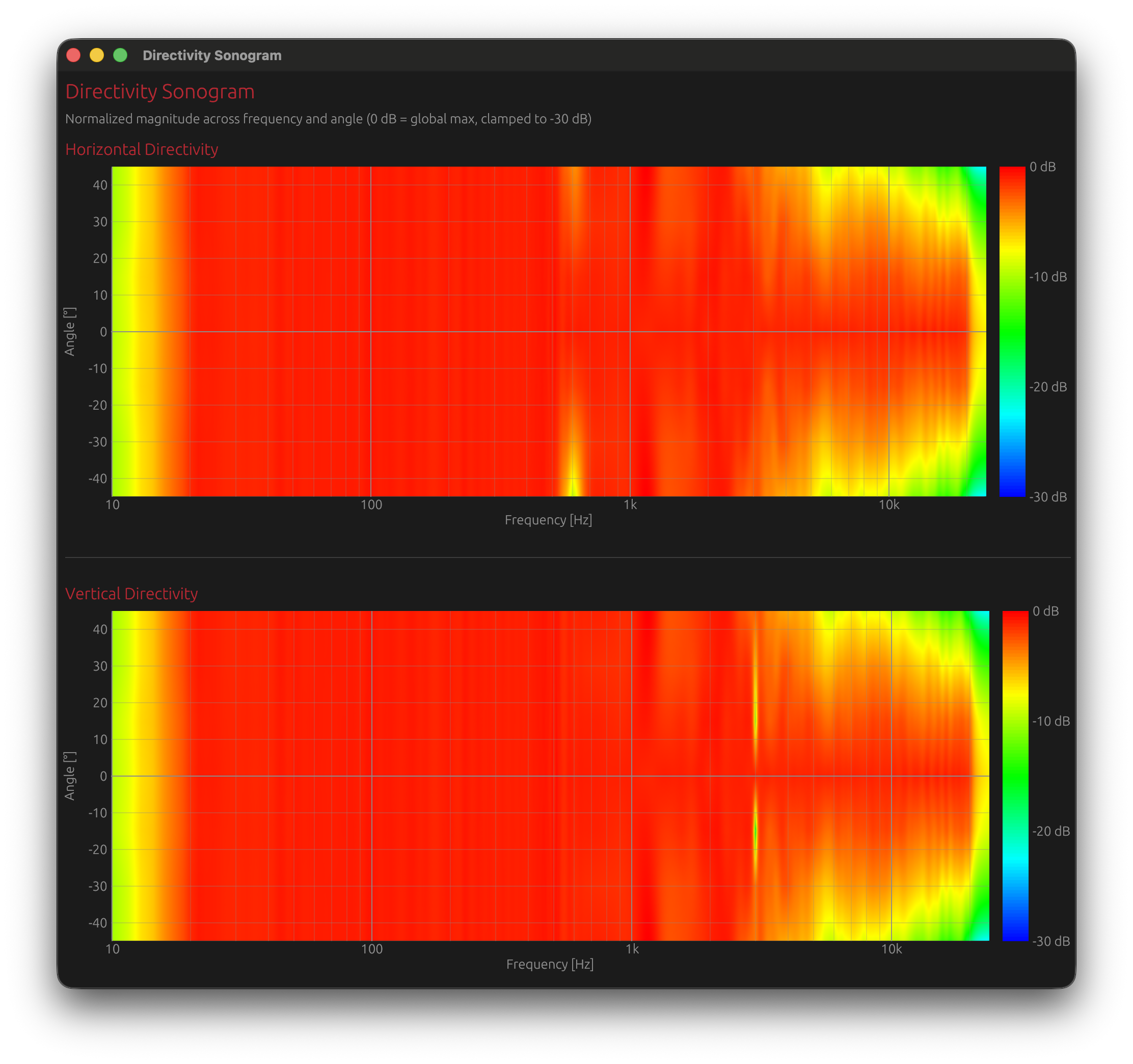
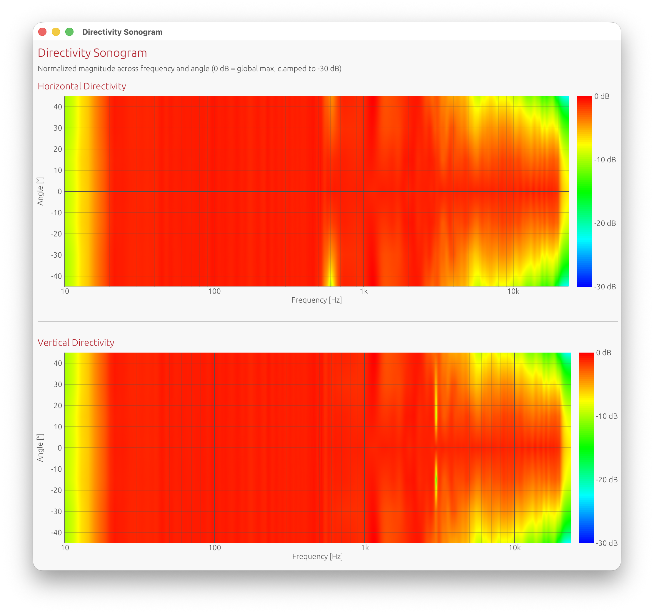
Directivity Sonograms
The Directivity Sonogram window displays 2D visualizations of how sound radiates across frequency and angle.
Accessing Sonogram Window
Menu: View → Directivity Sonogram
Requires: Valid LinFIR license and polar measurements loaded
Window Layout
Two separate sonogram plots:
- Horizontal directivity: Vertical angle = 0°, varying horizontal angle
- Vertical directivity: Horizontal angle = 0°, varying vertical angle
Axes:
- X-axis: Frequency (Hz, logarithmic scale)
- Y-axis: Measurement angle (degrees)
- Color: Normalized magnitude in dB (0 dB = global maximum)
Color Scale
Hot colors (red/yellow): Higher SPL (0 to -6 dB)
- On-axis or near-axis energy
- Focused radiation
Warm colors (orange): Moderate attenuation (-6 to -12 dB)
- Moderate off-axis output
- Typical dispersion
Cool colors (blue/purple): Significant attenuation (-12 to -30 dB)
- Heavily attenuated off-axis
- Beaming or nulls
Range clamped to -30 dB for clarity (adjustable in settings)
Interpreting Sonograms
Horizontal bands:
- Similar spectral balance across angles
- A band remaining coherent from about −60° to +60° indicates a well-designed driver with controlled directivity and no excessive beaming
Angular width and color spread:
- Warm colors extending from −90° to +90° in the bass / low-midrange are normal (low frequencies are inherently near-omnidirectional)
- Progressive narrowing at high frequencies is expected, but confinement to < −45° to +45° suggests excessive beaming
Symmetry around 0°:
- Geometrical and acoustical symmetry
- Proper driver placement and reliable measurements
Asymmetric patterns:
- Potential baffle diffraction
- Room reflections contaminating measurements
- Driver offset or asymmetric waveguides (intentional in most 3 way monitor designs)
Interference patterns (diagonal/complex):
- Driver interaction visible
- Crossover region summing effects
- Time-of-flight encoding driver spacing
What to Look For
Good Patterns:
Smooth color transitions:
- Gradual change from hot (on-axis) to cool (off-axis)
- Indicates controlled directivity
Symmetric patterns:
- Equal radiation to left/right (horizontal) or up/down (vertical)
- Indicates Symmetric design
Horizontal bands in crossover region:
- Consistent radiation pattern through crossover
- Good driver integration
Bad Patterns:
Narrow bright vertical regions:
- Beaming (concentrated energy on-axis)
- Excessive directivity at that frequency
- Often caused by large drivers at high frequencies
Dark spots off-axis / Diagonal stripes:
- Nulls or cancellations between drivers
- Indicates poor crossover alignment or lobing
- May be acceptable if smooth and symmetric
- Often caused by driver spacing and time-of-flight
- Crossover regions with insufficient acoustic slope, producing off-axis lobing
Crossover Design Insights
Compare on-axis and off-axis patterns:
- Check for consistent summing across all angles
- Look for lobing (bright spots appearing at off-axis angles)
Verify driver summing:
- Crossover frequency should show smooth transition in sonogram
- Moderate nulls or peaks appearing at specific angles
Adjust crossover if needed:
- Lobing visible: Try different crossover slopes or frequency
- Nulls visible: Check driver polarity and time alignment
Example Adjustments:
Problem: Bright and wide lobe at +30° near crossover frequency
Solution: Lower crossover frequency or increase slope to reduce overlap
Problem: Null at 0° (on-axis) at crossover frequency
Solution: Check driver polarity, adjust time delay, or change crossover type
Problem: Vertical bright bands alternating with dark bands
Solution: Driver spacing issue (comb filtering) - may require physical redesign
Why Time-of-Flight Matters
Physics of Multi-Driver Interference
When multiple drivers reproduce the same frequency range, their outputs combine in space. The phase relationship between drivers depends on:
- Physical separation between drivers (geometry)
- Acoustic path length differences to the measurement point
- Crossover filter phase shifts
How Time-of-Flight Encodes This
Each driver’s impulse arrives at a slightly different time:
- This delay represents the acoustic path length to the microphone
- At the on-axis position, path lengths may be similar
- At off-axis positions, path length ratios change
Off-axis measurements capture geometry:
- Driver A might be 1.0 meters away on-axis
- Driver B might be 1.05 meters away on-axis (5 cm path difference)
- At +30° off-axis, Driver A might be 0.95 m and Driver B might be 1.15 m (20 cm difference)
- This changing path length ratio creates interference patterns
These delays create directivity:
- At some frequencies, drivers sum constructively (in phase)
- At other frequencies, drivers sum destructively (out of phase)
- The frequency where this happens depends on the angle (because path lengths change with angle)
- This is the fundamental physics of directivity
What Happens If You Remove TOF without keeping relative delays
Time-aligning removes geometric delay information:
- All drivers appear to arrive at the same time
- DI calculation assumes drivers are co-located (all at the same point in space)
- This is physically incorrect for real speakers
Predicted interference patterns don’t match reality:
- Off-axis nulls and peaks won’t appear
- Directivity sonograms show incorrect lobing
- DI curve does not reflect actual radiation pattern
Example:
With TOF preserved:
- Tweeter and woofer are 15 cm apart vertically
- At 2.3 kHz (wavelength ≈ 15 cm), expect null at certain off-axis angles
- DI curve shows this correctly
With TOF removed (time-aligned):
- Software thinks drivers are co-located
- Predicts no null at 2.3 kHz
- DI curve is smooth (incorrect)
- Real speaker still has null at 2.3 kHz off-axis
Proper Workflow
1. Capture IR with full time-of-flight intact
- Use proper timing reference (electric loopback or acoustic chirp)
- Do not apply windowing that removes acoustic delay
- Preserve the natural arrival time differences
2. Import into LinFIR preserving the delay
- Keep the raw impulse peak positions as captured or remove the same amount of time across all measurements
- Each angle will have slightly different delay values (this is correct)
3. Apply crossover filters
- Crossovers add their own phase shifts
- These combine with geometric delays
4. LinFIR predicts directivity
- Calculation includes both geometry (TOF) and filtering (crossover phase)
- Spherical integration over all measured angles
- Result: realistic DI and sonograms
5. Sonogram shows realistic interference
- Interference patterns reflect both driver spacing and crossover design
- Allows optimization of crossover for desired directivity
Limitations and Best Practices
Measurement Density
More angle measurements = more accurate prediction
- Minimum recommended: 7 angles per axis (±90° in 30° steps)
- Good: 13 angles per axis (±90° in 15° steps)
- Ideal: 19 angles per axis (±90° in 10° steps) or finer
Why density matters:
- DI calculation uses spherical integration
- Sparse measurements = poor integration accuracy
- Fine measurements = more accurate directivity prediction
Room Reflections
Directivity analysis is most accurate in anechoic conditions
- Room reflections distort off-axis measurements
- Early reflections appear as interference in the sonogram
- Can create false lobing patterns
Mitigation strategies:
- Measure outdoors (less reflections)
- Measure in large room with speaker away from walls
- Use gating/windowing carefully:
- Remove late reflections (>10 ms after main arrival)
- Use Adaptive Window to preserve bass while gating reflections
Microphone Position
Keep measurement distance constant:
- Same distance for all angles
- Ensures consistent SPL normalization
- Eliminates distance-related level variations
Farfield measurements (>1 meter) work best:
- Avoids nearfield effects
- Drivers behave as coherent sound sources
- More accurate directivity prediction
Microphone height:
- Should match speaker acoustic center
- For 2-way speaker, typically between tweeter and woofer
- Ensures symmetric vertical measurements
Computational Notes
DI calculation uses spherical integration:
- Computationally intensive (integrates over all angles and frequencies)
- May take a few seconds for dense polar data
Sonogram generation:
- Creates high-resolution 2D images (frequency × angle)
- Parallel processing used for speed
- Results are cached to improve performance
Getting a License
To unlock Directivity Analysis tools:
- Visit the LinFIR website: https://linfir.demaudio.com
- Purchase a license key
- Enter your e-mail and key in LinFIR: Settings → License
- All directivity features will be enabled immediately
Your license supports:
- Ongoing development
- New features
- Bug fixes and improvements
Related Documentation
- IR Management: Capturing and managing off-axis measurements
- Audio Setup: Configuring audio interface, measurement settings, and timing reference for accurate polar measurements
- Driver Processing: Crossover design and optimization
Summary
Directivity Analysis tools characterize how your speaker radiates sound in different directions:
Features:
- Off-axis frequency response visualization at any angle
- Directivity Index (DI) prediction across the spectrum
- Directivity sonograms (2D frequency vs. angle heatmaps)
Requirements:
- Valid LinFIR license
- Polar measurements at multiple angles (horizontal and vertical)
- Preserved time-of-flight
- Proper timing reference (electric loopback or acoustic chirp)
Key Concepts:
- Time-of-flight encodes driver geometry (must be preserved)
- DI quantifies how directional the speaker is (0 dB = omni, higher = more directional)
- Sonograms visualize radiation patterns (hot colors = on-axis energy, cool = off-axis attenuation)
- Crossover optimization based on directivity for consistent off-axis response
Workflow:
- Configure timing reference (electric loopback recommended)
- Capture polar measurements for each drivers (preserve time-of-flight)
- Design crossovers and apply filters
- View off-axis curves, DI, and sonograms
- Optimize crossover for desired directivity pattern
- Iterate based on measurements
Use directivity analysis to understand and optimize your speaker’s radiation pattern for better room interaction and consistent sound across the listening area.