Near-Field / Far-Field Splicing 🔒
License Required: The splicing wizard requires a valid LinFIR license.
The splicing wizard synthesizes a full-range anechoic response for a loudspeaker by combining near-field captures of each radiating element (driver, vent, passive radiator) with the far-field polar measurements you already have for the same driver. It follows the method popularized by Don Keele: near-field measurements are immune to the room but only valid at low frequencies, far-field measurements carry the real directivity and diffraction but can’t be gated long enough to stay clean in the bass — the wizard splices the two in a transition band so the strengths of each cover for the weaknesses of the other.
The result replaces the raw far-field capture, for every measured angle, everywhere it is used in LinFIR (response, DI, sonogram, exports).
This page describes the wizard step by step. For the window it lives in, see IR Management — the wizard is reached from the Near-field measurements (splicing) section there.
When to Use It
Use splicing when your far-field measurements are not anechoic down to the bottom of the passband — which is almost always the case indoors:
- A far-field measurement gated to keep the first room reflection out is only trustworthy above roughly
1000 / gate_msHz (a 5 ms gate → ~200 Hz). - Below that, the gate is shorter than one period and the low end is unusable.
- Near-field measurements fill that gap: with the mic almost touching the cone, the direct sound is ~40 dB above the room, so no gating is needed.
You do not need splicing if you measured outdoors / ground-plane / in an anechoic chamber and your far-field response is already clean to 20 Hz.
What You Need Before Starting
- An on-axis (0°, 0°) far-field measurement for this driver, imported or captured in IR Management. The wizard blends against it (and against every other stored angle when you finalize).
- Near-field access to every radiating element. For each one you’ll place the mic a few millimetres from:
- the dust cap / cone of each driver,
- the mouth of each vent (port),
- the diaphragm of each passive radiator.
- The element’s effective radiating area Sd (cm²) — from the datasheet, or
π·(effective radius)². - The enclosure dimensions and where each element sits on it.
- The same gain chain and sweep parameters for every near-field capture. The relative levels between elements are physically meaningful; changing input gain between captures silently invalidates them and cannot be corrected afterwards.
⚠️ Passive radiators and vents produce a weak near-field signal away from tuning. The wizard’s captures deliberately do not reject a low-level sweep — judge the level from the meter and the IR/FR preview instead.
Opening the Wizard
IR Management → Near-field measurements (splicing) → Open splicing wizard…
The button is disabled until an on-axis far-field measurement exists, and (with no license) shows “requires a valid license” on hover. The wizard opens in its own window with a tab strip for the seven steps. Navigation is free — you can jump back to any earlier step and change something without redoing captures already taken; every later plot recomputes automatically.
Step 1 — Near-Field Elements
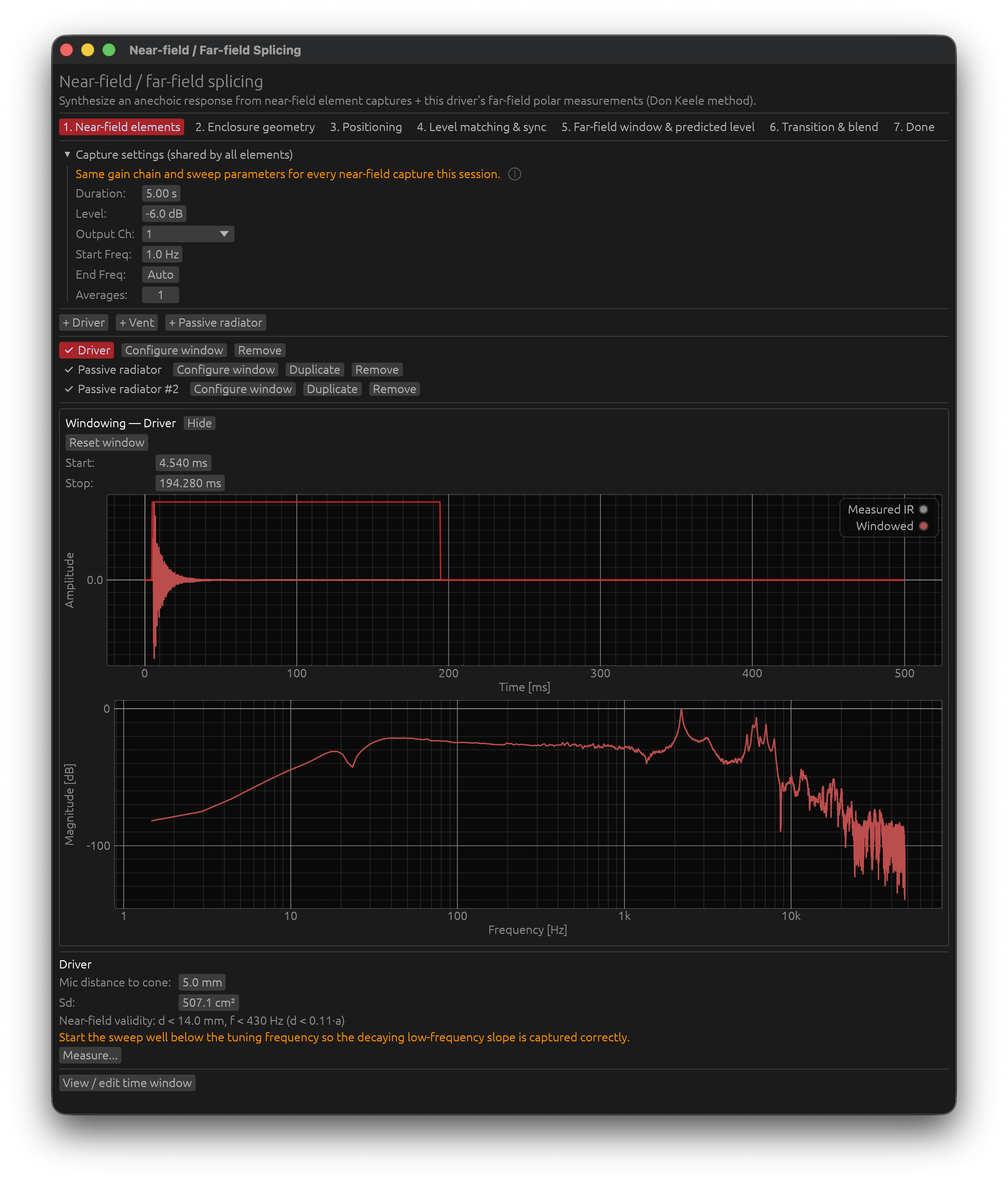
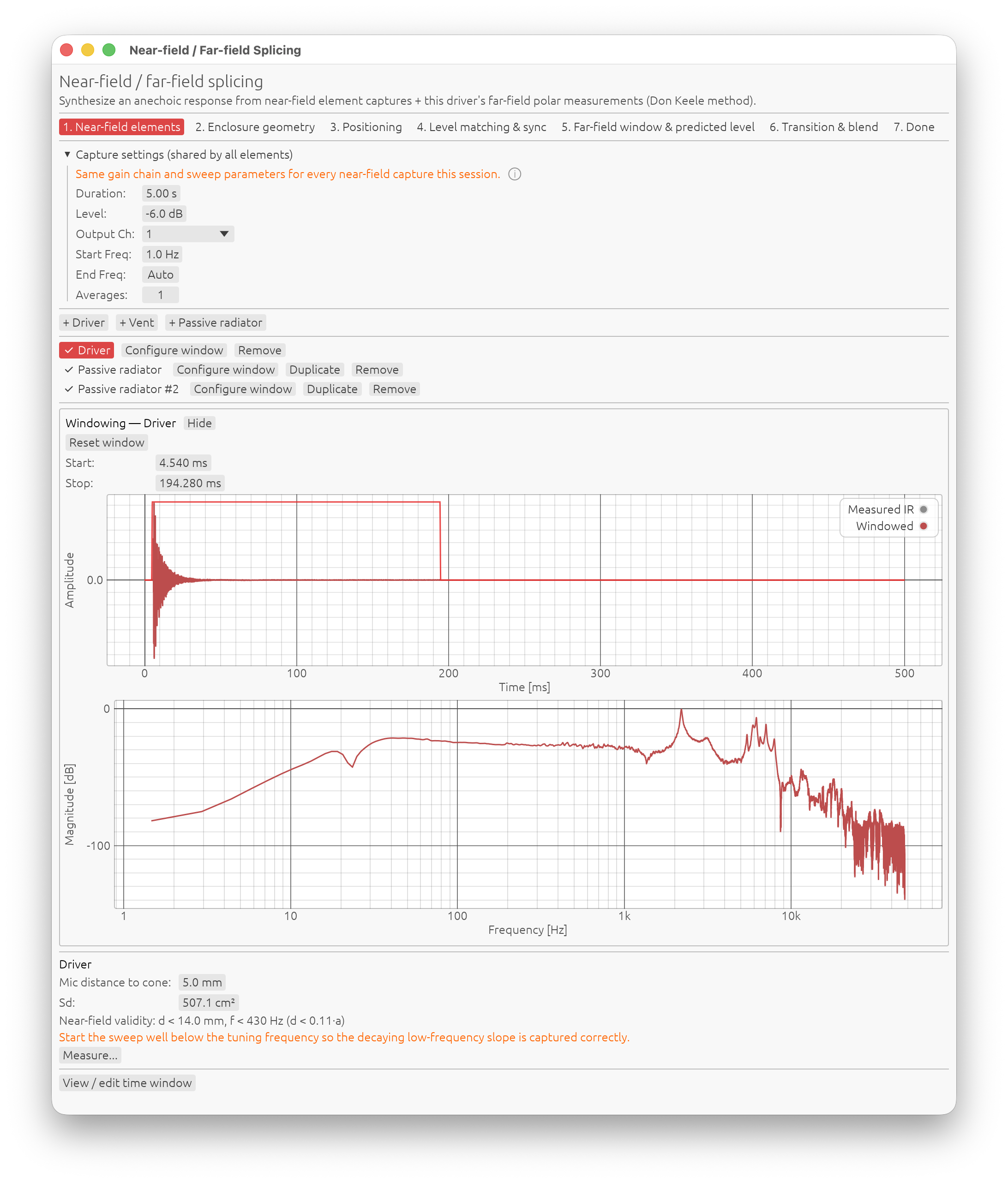
Add one element per radiating surface and capture its near-field impulse response.
Adding elements
- + Driver, + Vent, + Passive radiator — one element per physical radiating part, not per way (a “way” is a frequency band, not a driver count): add one Driver for every driver unit on the enclosure, even if several share the same band — a 2-way MTM/D’Appolito (two identical woofers plus one tweeter, still only two ways) is three drivers. Add one Vent per port and one Passive radiator per drone. A sealed 2-way with a single woofer is two drivers, no vent; the same box ported is two drivers + one vent; an isobaric-loaded sub with two drones is one driver + two passive radiators.
- Each element gets a status marker: ○ not measured, ✅ measured.
Per-element settings
| Field | What to enter |
|---|---|
| Mic distance to cone / baffle surface | The actual measured distance, in mm. Keep it small. |
| Sd | Effective radiating area in cm². Required even for vents and passive radiators. |
Below the fields, the wizard shows the near-field validity limits for that Sd:
d < 0.11·a— the mic must be closer than this or the reading isn’t a true near-field pressure (a= equivalent piston radius from Sd).f < c / (2·√(π·Sd))— above this frequency the near-field assumption breaks down (it corresponds toka = 1; the appendix explains the physics). For a 6½″ driver this is around 1 kHz; for a 15″ woofer, around 350 Hz; for a large passive radiator, lower still. This is the ceiling of what the splice can take from the near field — the transition band must sit below it.
Capturing
Measure… runs a sweep with the shared parameters (set in the wizard’s Capture settings header — duration, level, start / end frequency, averages). Watch the level meter — aim for a healthy but unclipped level. For a passive radiator or an off-tuning vent, a low reading is normal and is not rejected.
The near field only feeds the splice below the ka = 1 limit above, so a full-bandwidth sweep is rarely needed here. If an element has a loud out-of-band resonance that forces you to drop the level, lower the End Freq below it (see Sweep Measurements) so the useful band gets full level.
Windowing each capture
After a capture, View / edit time window (also reachable any time via Configure window in the element list) opens the per-element windowing editor:
- Start / Stop in ms, with the same raised-cosine (Tukey) taper the main IR window uses.
- The measured IR is shown with the windowed result and a red window-envelope overlay that holds for 3 s then fades — exactly like the main window’s time graphs.
- Reset window restores the full length.
Advice: near-field captures are already clean, so window loosely. Keep the start at 0 ms (or just before the peak) and set the stop well after the decay has died — a near-field port resonance rings for a long time and you want all of it. Cutting the tail short rolls off the very bottom of that element’s response.
Step 2 — Enclosure Geometry
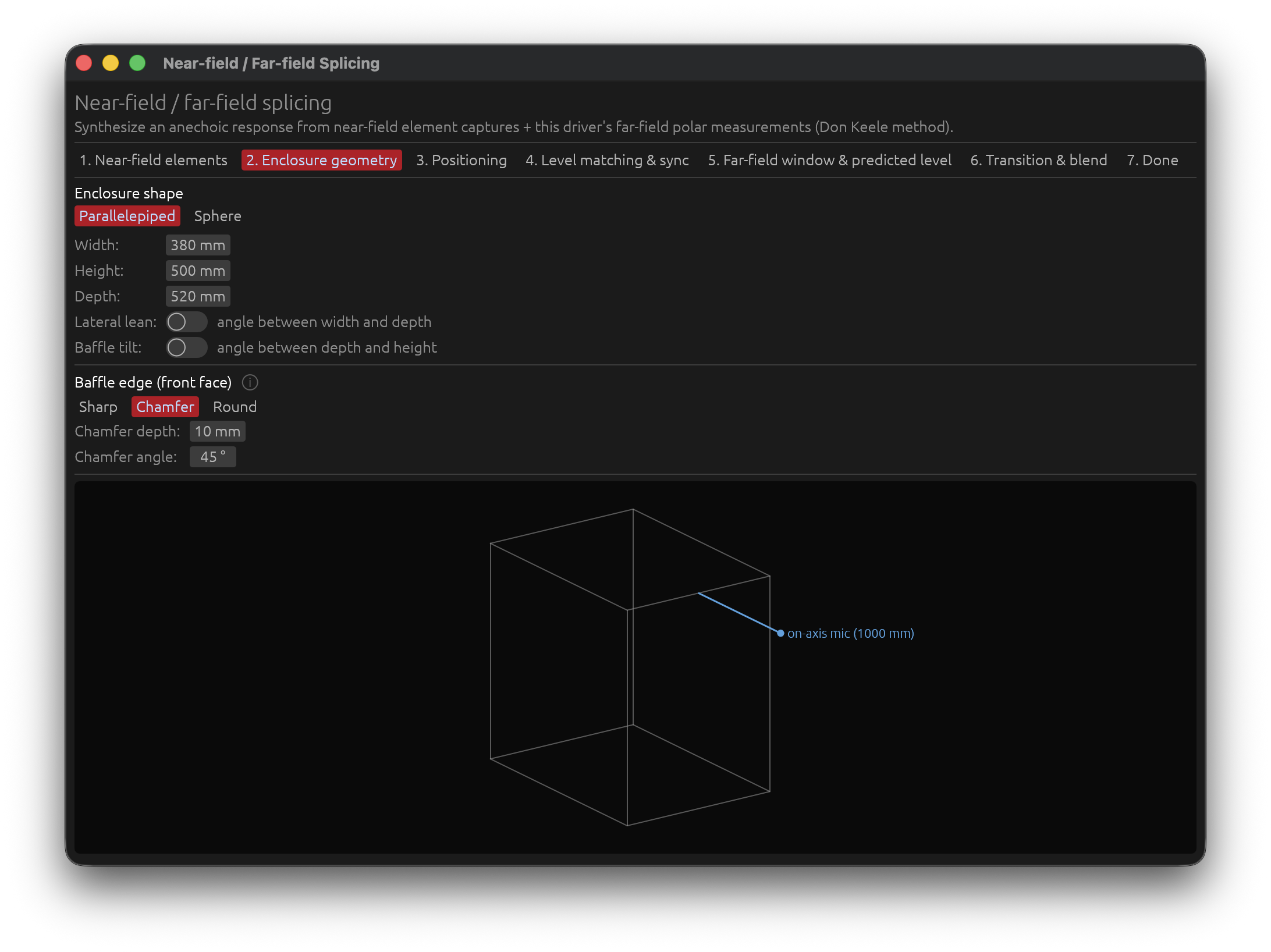
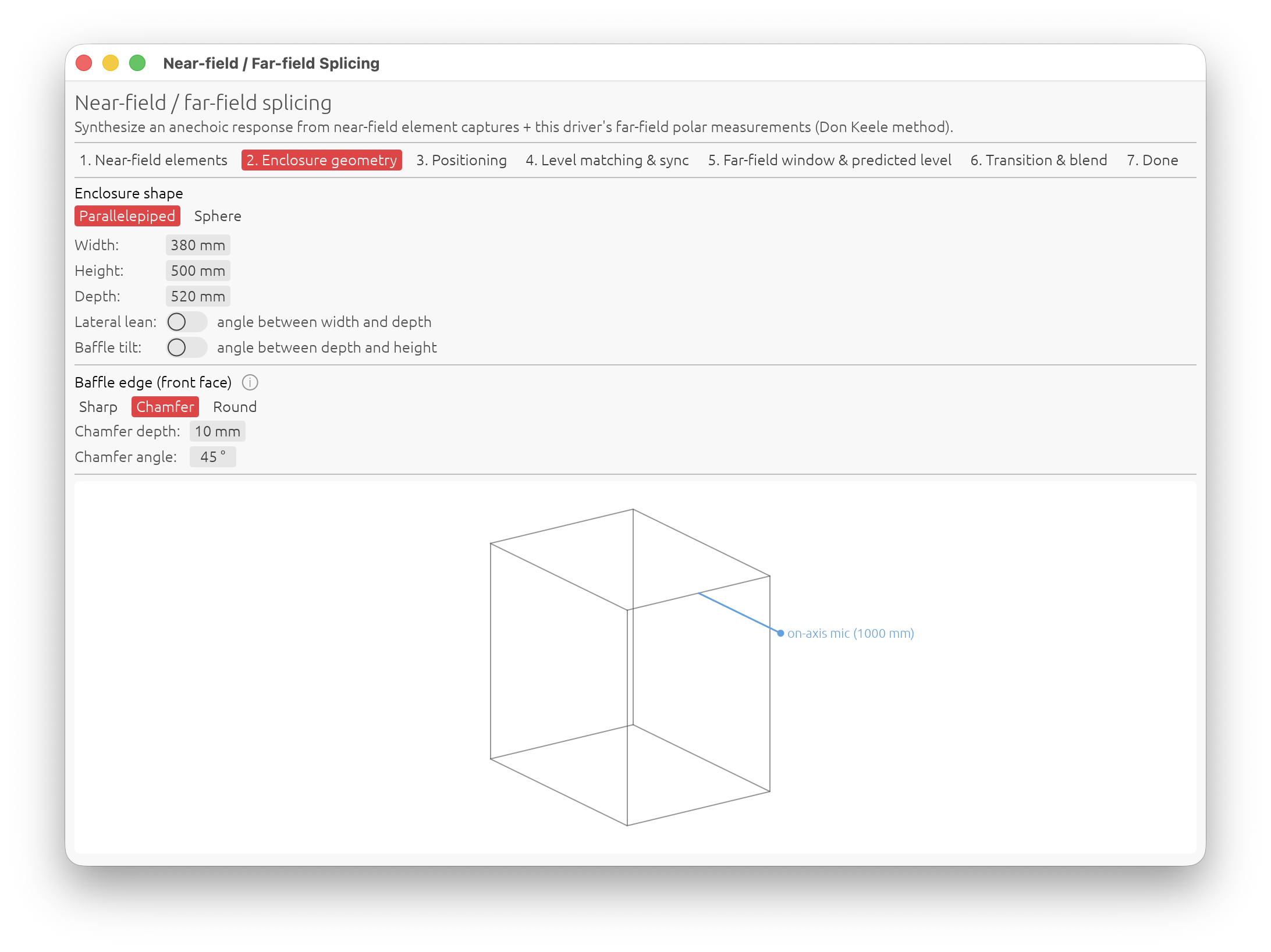
The geometry feeds the diffraction and time-of-flight model. It does not have to be a perfect 3-D replica — it has to get the baffle size, the element positions relative to the edges, and the mic direction right.
Enclosure shape
- Parallelepiped — width × height × depth in mm, with two optional shape angles:
- Lateral lean (angle between width and depth) — shears the box sideways. The front face stays perpendicular to the on-axis direction, so this does not change the acoustic axis; it mainly affects wrap-around diffraction to the sides.
- Baffle tilt (angle between depth and height) — rotates the front baffle about its horizontal centreline, so the baffle is inclined relative to the on-axis direction (a leaning cabinet). Positive = baffle aimed upward, top edge back. Your on-axis far-field measurement already saw the baffle at this angle, so entering it here keeps the predicted and measured responses consistent. The distance reference stays where the on-axis line meets the tilted face.
- Sphere — a single radius. No edges: the model uses a smooth 4π→2π radiation-loading transition instead of edge diffraction.
A more general enclosure shape (arbitrary hexahedron / tapered cabinet) is planned for a later version.
Baffle edge (front face)
- Sharp, Chamfer (depth + angle), or Round (radius).
- Chamfer / round are approximated as extra offset edges in the front-face diffraction model. The wireframe preview always draws a sharp edge regardless.
Advice: the baffle-step frequency and the diffraction ripple depend mostly on the baffle width and the driver’s offset from the nearest edges, so measure those carefully. Edge treatment is a second-order refinement — get it roughly right and move on.
Step 3 — Positioning
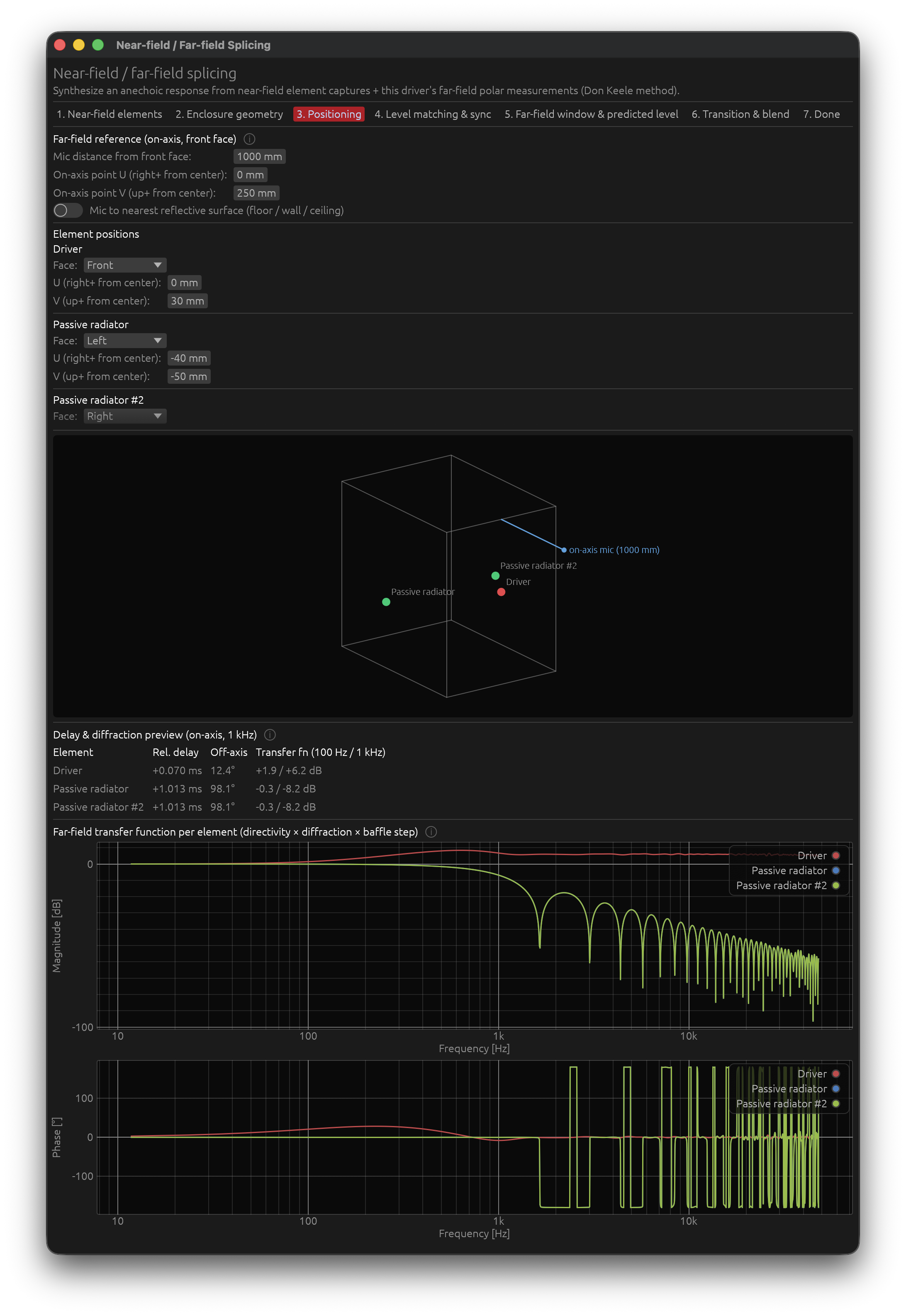
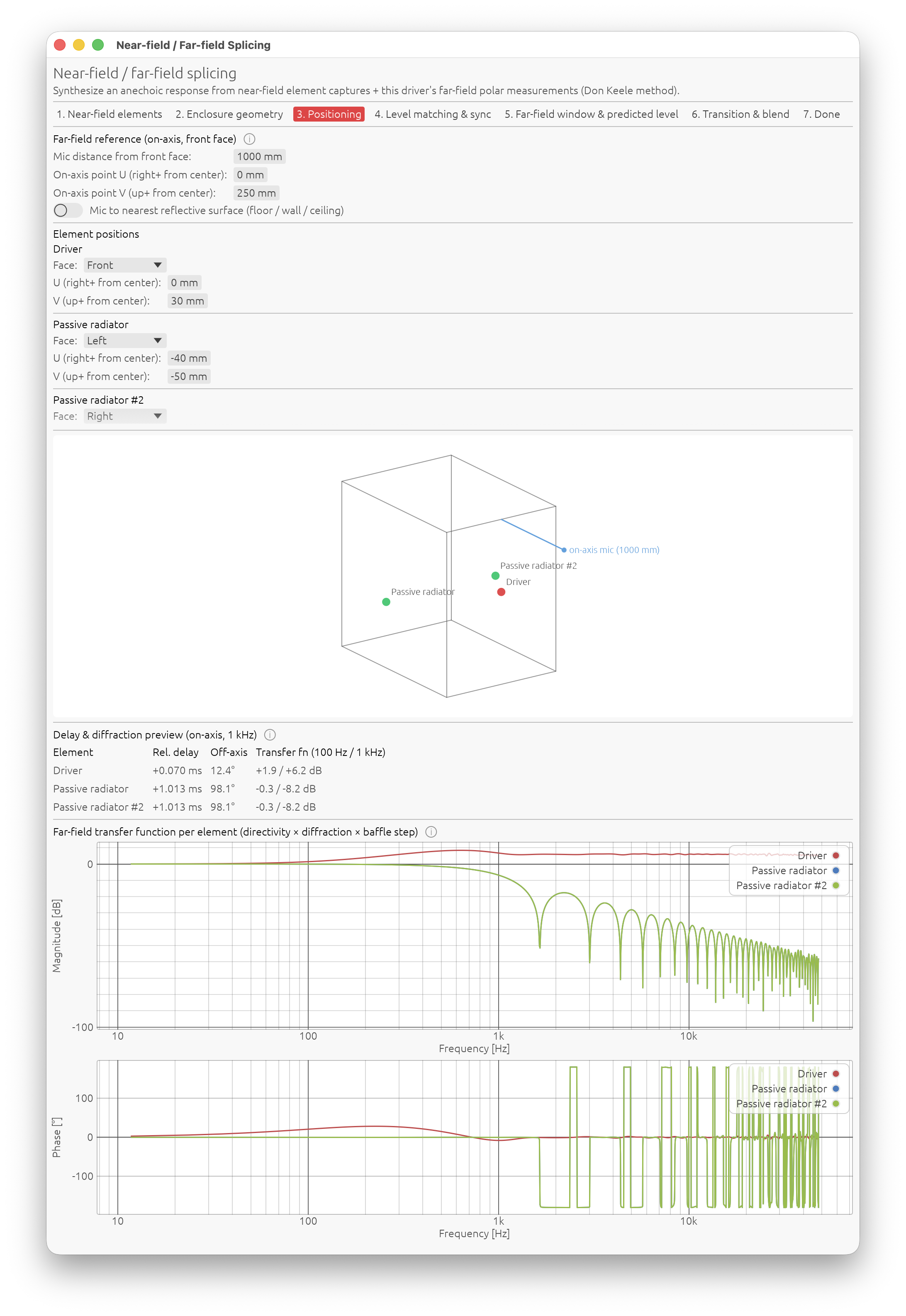
Far-field reference (on-axis, front face)
- Mic distance from front face — the distance your far-field polar set was measured at.
- On-axis point U / V — where the mic was aimed, relative to the front-face centre (0/0). This is normally 0/0, or the offset of an off-centre tweeter. It can be pushed outside the baffle for an off-axis or ground-plane sub measurement.
Mic to nearest reflective surface (image-source guard)
Optionally enter the perpendicular distance from the mic to the closest floor, wall or ceiling. From that plus the mic distance the wizard computes, via the image-source method, when the first room reflection arrives:
$$\Delta t = \frac{\sqrt{D^2 + 4h^2} - D}{c}$$
(D = mic distance, h = mic-to-boundary distance). It then:
- shows the arrival time and the lowest frequency the far-field capture stays reflection-free at,
- warns on Step 5 if your far-field window reaches past that gate,
- warns on Step 6 when the reflection — not the window length — is what prevents the near- and far-field bands from overlapping, and tells you to re-measure further from the walls.
Element positions
For each element, set its face (Front / Back / Left / Right / Top / Bottom) and its U / V position on that face in mm from the face centre. A vent or passive radiator on a side, top, bottom or rear panel is handled correctly — it diffracts around that panel’s edges, with its dipole axis perpendicular to that panel.
The oblique wireframe preview shows the box with coloured markers for each element and the mic.
Delay & diffraction preview
A table showing, per element, at the on-axis mic:
- Rel. delay — geometric time-of-flight relative to the rotation point.
- Off-axis — the angle from the element’s normal to the mic.
- Transfer fn (100 Hz / 1 kHz) — the diffraction + directivity gain in dB.
Far-field transfer function per element
Two plots (magnitude + phase) of the geometry-only shaping each element’s radiation undergoes on the way to the far-field mic — the Distributed Edge Dipole model: intrinsic piston directivity, driving-pressure obliquity, and edge dipoles. This is not multiplied by the element’s own measured response, gain or propagation delay — it is purely the per-element multiplier the predictor applies before summing.
DC-normalized to 0 dB (the standard diffraction-response convention): flat near 0 dB below the baffle-step corner, rising toward +6 dB with ripple above it. Phase excludes the geometric delay.
Advice: use these plots to sanity-check the geometry. On axis, an element centred on the baffle should sit near 0 dB in the bass and climb smoothly. A wildly rippled or lopsided curve usually means a wrong dimension or a mis-placed element.
Step 4 — Level Matching & Sync
This step only appears when there’s something to do on it: the enclosure has a vent or passive radiator (level matching), or more than one element was captured (sync alignment). A sealed, single-driver box has neither and skips straight to Step 5.
The relative level between the driver(s) and the vent(s) / passive radiator(s) is set from physics — each element’s Sd and its measured mic distance — not by curve-fitting. If those were measured accurately, no adjustment is needed.
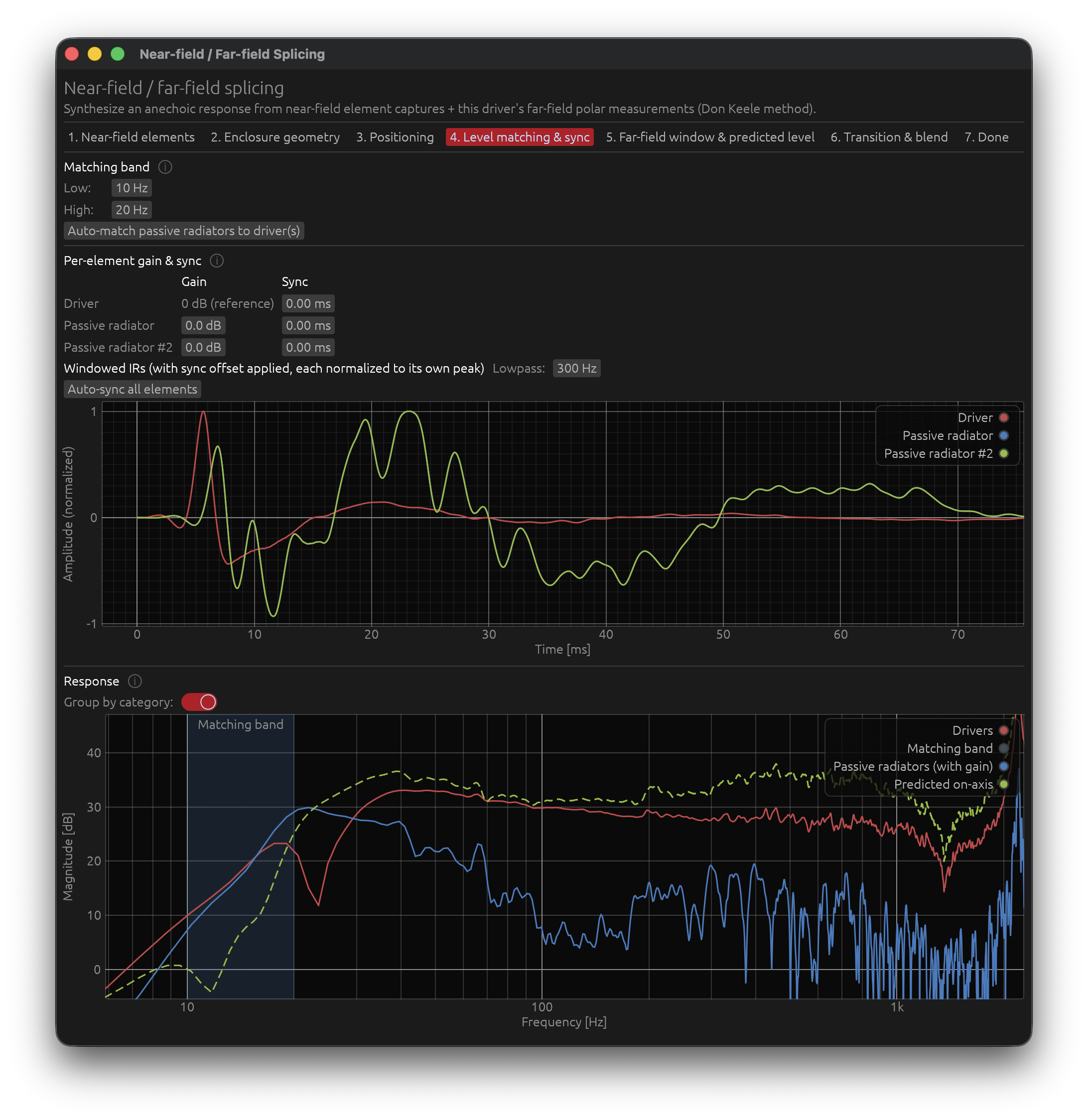
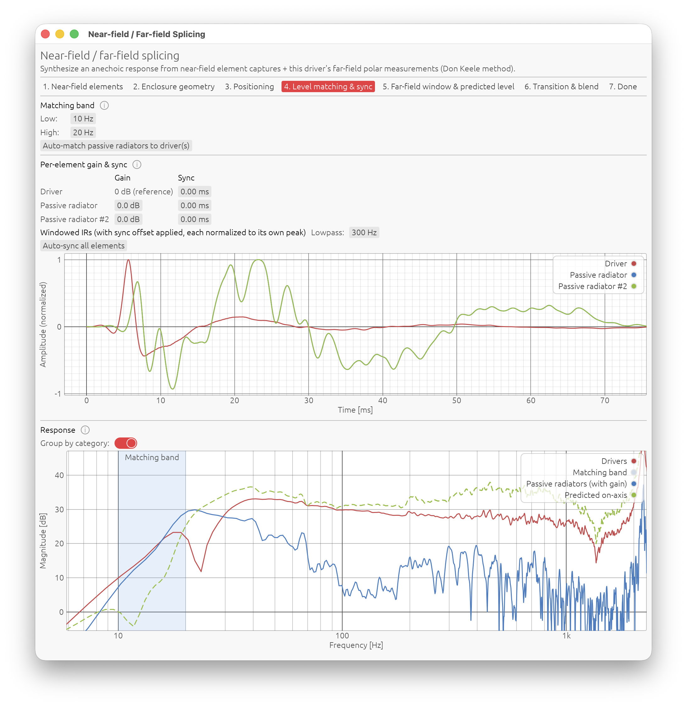
Matching band
Pick the lowest, straight-sloping part of the spectrum, below the box tuning frequency, with the Low / High fields. This band is used for the comparison and for auto-match.
Auto-match
Auto-match … to driver(s) shifts the non-driver elements’ gain so their combined level equals the driver level over the matching band.
⚠️ Auto-match fits the band by curve shape. That is valid for a vent (its near-field curve runs tangent to the driver’s near tuning) but not for a passive radiator — a PR’s near-field curve crosses the driver’s. Auto-matching a PR can paper over a real Sd / distance measurement error. For a PR, prefer the manual gain.
Per-element gain & sync
The sync column only appears when more than one element was captured.
One grid, two purposes:
-
Gain — a dB trim per non-driver element. 0 dB = trust the Sd / distance figures. Only touch it if you don’t trust those measurements (or after Auto-match above).
-
Sync — a timing correction (ms) per element, positive delays it further. Leave every offset at 0 if the measurement chain was correctly synchronized — a hardware (Electric) timing reference (see Audio Setup) for every capture — there’s nothing to fix.
Without Electric sync — most commonly because the measurement microphone is a USB device with its own independent clock, which precludes any electrical or acoustic loopback — elements are captured as separate sweeps with no shared clock between the output and the microphone’s own capture stream, so ordinary capture-chain jitter between one capture and the next can misalign them enough to corrupt the complex sum below: an artificial notch or bump appears where there shouldn’t be one, or an existing one is exaggerated. Lowpass and Auto-sync all elements, below, are the tools for fixing that.
Lowpass
Next to the Windowed IRs plot. Display only — it never touches the splice recipe: a 4th-order-Butterworth-shaped, linear-phase FIR (10 001 taps, exactly delay-compensated so the trace’s own timing doesn’t shift as you move the slider), for cleaning up the trace before aligning anything, whether by eye or with Auto-sync below.
Set it well above the box tuning frequency. The goal is to strip whatever masks the driver/vent-PR working zone — cone breakup, resonances, the part of the spectrum each element doesn’t share with the others — not to zoom into the sub-bass alone. Cutting too close to tuning throws away the very region you’re comparing.
Manual alignment
With the traces cleaned up by Lowpass, align the main peaks on the Windowed IRs plot by eye, by group:
- Several drivers — they’re driven identically, so their captured phase should coincide. Bring them into alignment with each other first.
- Several vents, or several passive radiators — same idea: align each one against another of its own kind.
- Driver(s) vs vent(s)/passive radiator(s) — once each group is internally aligned, shift the whole group against the other. Correct relative timing makes the summed magnitude smooth (even a slight rise) around the box tuning frequency; wrong timing punches an artificial notch there instead.
⚠️ With a correct Electric sync, don’t chase a pixel-perfect overlap for step 3. You’ll normally see the driver and vent/PR peaks very slightly offset yet still overlapping — that’s expected, not an error. It comes from the driver and the vent/PR being physically apart, combined with the passive element’s own reaction time (it isn’t driven electrically, so it genuinely takes a little longer to start moving). Forcing that residual to exactly zero would erase real, physical information from the splice.
Auto-sync all elements
Does the above automatically, in one click, for sessions with no reliable timing reference at all: aligns the first significant peak of every element’s lowpass-filtered IR to the first captured element’s, replacing each other one’s Sync offset with the result. The reference element is left untouched. Re-run after changing the Lowpass cutoff if the result looks off, or fall back to the manual steps above if it doesn’t.
It aligns everything, including driver against vent/PR — unlike doing step 3 by hand, it doesn’t leave the small physical residual from the warning above; that’s an accepted trade-off for a one-click bulk fix (jitter with no reference at all can run to many milliseconds, dwarfing that residual). Nudge the relevant Sync field afterward if it matters for your enclosure. With a correct Electric sync, don’t use this button at all - there’s nothing to fix.
Response
- Group by category — off by default (one curve per element); switch on to sum all drivers into one curve and all vents/passive radiators into another instead, matching the two contributions the matching band and Auto-match above actually compare — fewer curves, at the cost of losing the per-element detail.
- Individual element curves (default) — each element’s own near-field magnitude (Sd / distance-corrected and gained, no diffraction). They should be close to each other over the matching band; the band readout (shaded) gives the exact Δ in dB.
- Predicted on-axis (dashed) — every positioned, captured element delayed by its geometry, shaped by its directivity and baffle diffraction, then summed as complex responses, so the driver / vent phase relationship — anti-phase below tuning, in-phase through the passband — is preserved. Check it for a smooth transition (no artificial notch) around the box tuning frequency. A warning lists any element left out of the sum for want of a position or a capture.
Step 5 — Far-Field Window & Predicted Level
Far-field on-axis time window
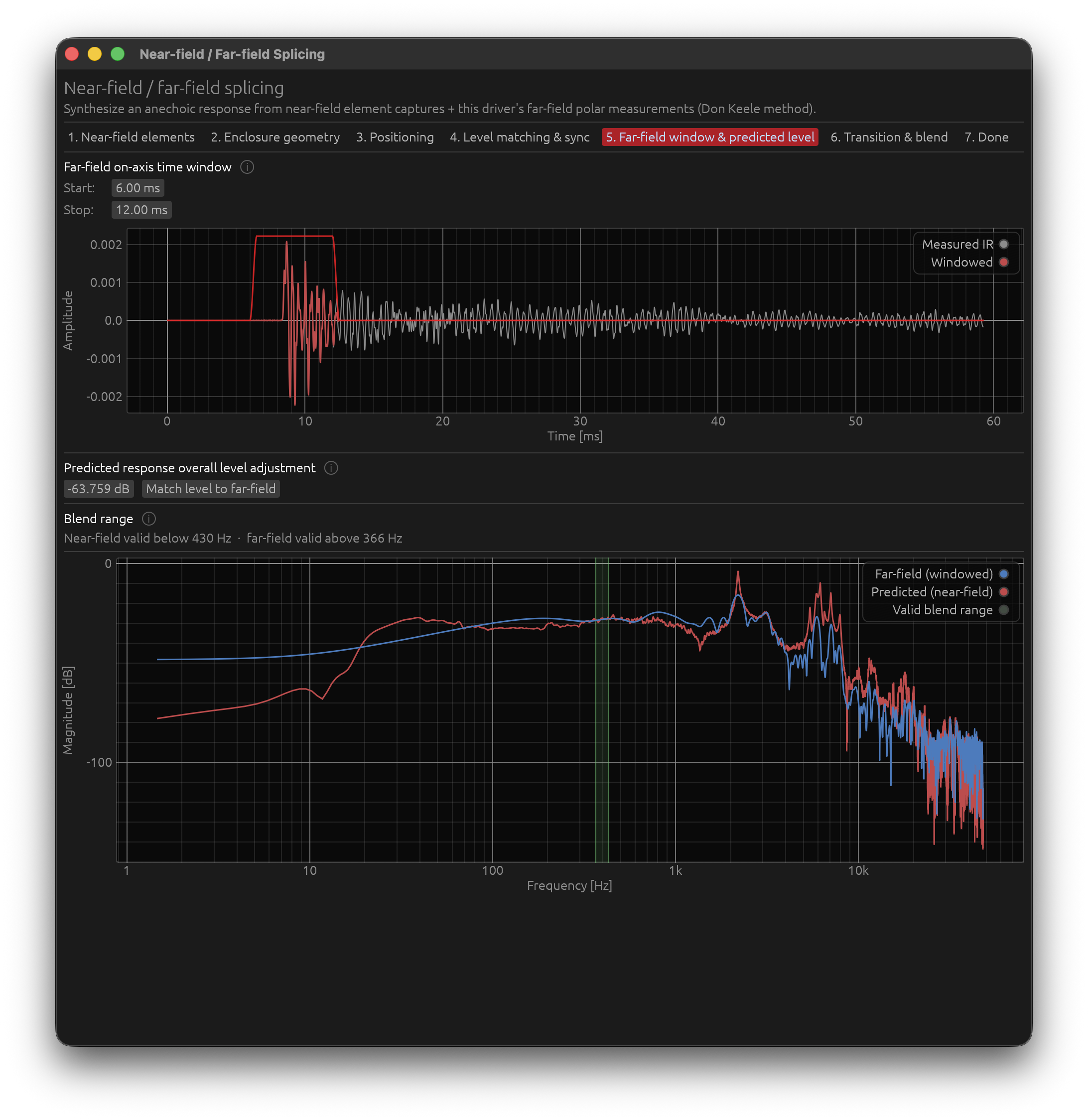
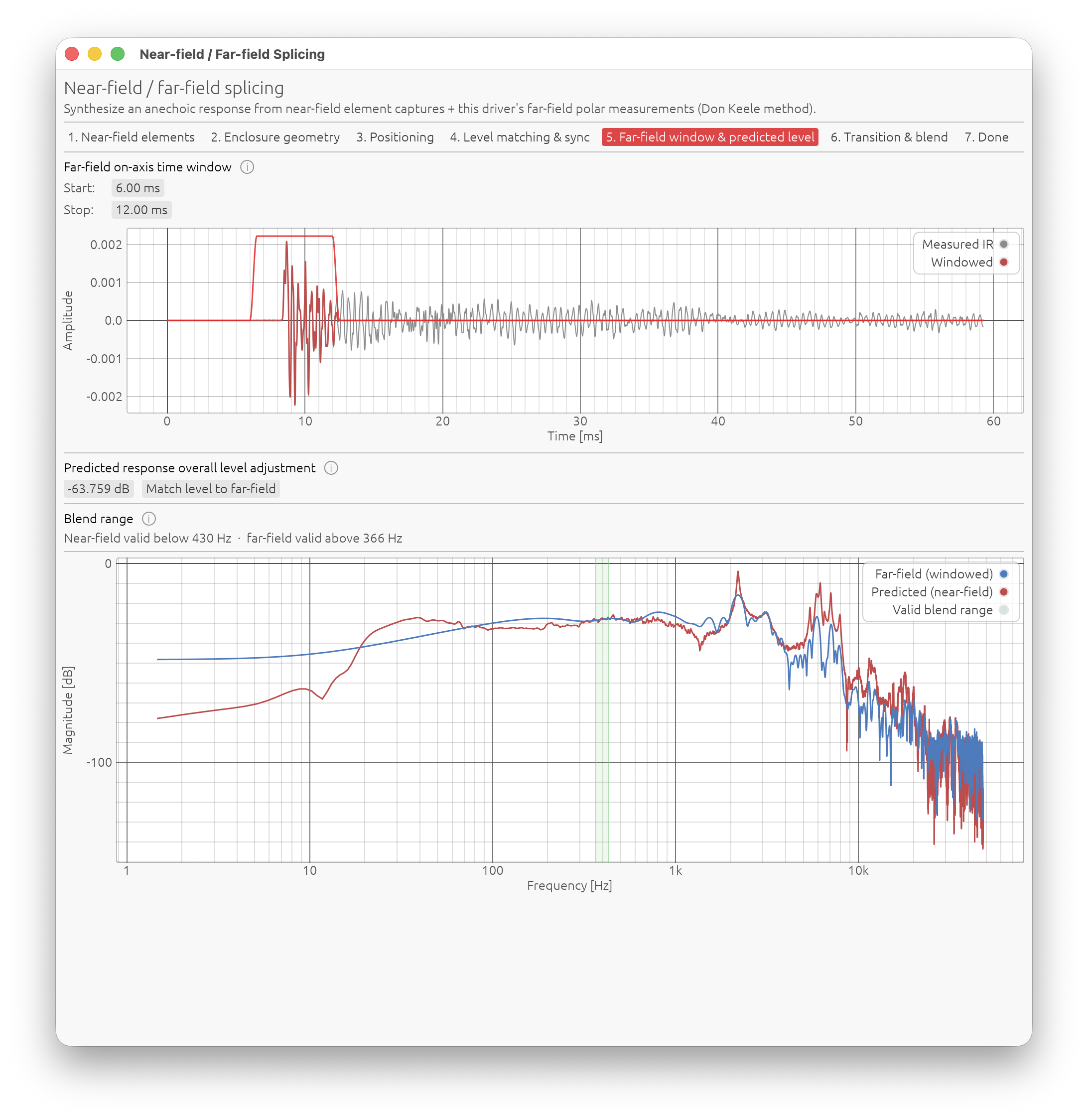
A simple window on the raw far-field capture, bypassing the driver’s own configured windowing (which is tuned for the final crossover-ready response, not for this splice).
- Start / Stop in ms.
- The time-domain plot below shows the measured IR, the windowed result and — while you drag — a fading red window-envelope overlay, the same as the per-element view on Step 1. Room reflections show up as bumps after the direct-sound peak; set Stop just before the first one.
- If you entered a mic-to-boundary distance in Step 3, a dashed orange “First reflection” marker shows where the image-source model expects that reflection, and a red warning appears if the window runs past it (with the exact Stop time to use).
Advice: window as long as the room allows without letting a reflection in — a longer far-field window lowers the far-field floor, which widens the valid blend range. When a clean reflection isn’t visible, trust the marker.
Predicted response overall level adjustment
A dB offset that lines the predicted near-field curve up with the far-field measurement across the valid blend range (green).
There is no reliable absolute reference between the two sets — you typically change gain-chain settings between near- and far-field sweeps (to avoid saturating the mic up close) — and the Sd / distance physics already scales each element’s near-field capture by up to Sd itself (tens of dB), so the value you need here can be far larger than a normal trim. That is expected.
Match level to far-field — next to the offset — sets it automatically: it shifts the predicted curve onto the windowed far-field measurement across the valid blend range, using the median of the per-bin level difference (median rather than mean so a diffraction ripple or a narrow notch near a band edge doesn’t drag the match off). Use it as a starting point, then nudge the offset by hand if the two curves still cross rather than run parallel. It needs a far-field window and at least one captured element; if there is no valid overlap it falls back to the configured transition band.
Blend range
The valid blend range is where the two measurements overlap and can be blended:
- the near field is valid below its ceiling
c / (2·√(π·Sd))(smallest element — see the appendix); - the far field is valid above its floor — the more restrictive of the window-length limit (
1000 / (window_stop − peak)) and the room-reflection limit.
A readout shows both limits, and the compare plot shades the overlap in green (“Valid blend range”). Lengthening the far-field window lowers the floor and widens the range; if the floor ends up above the ceiling there is no overlap and a red message tells you what to do.
The transition band itself (where inside this range the crossover sits) is set on the next step.
Advice: window the far field as long as the room allows and set the level so the two curves sit on top of each other across the green range. That is what makes Step 6 easy.
Step 6 — Transition & Blend
Transition band
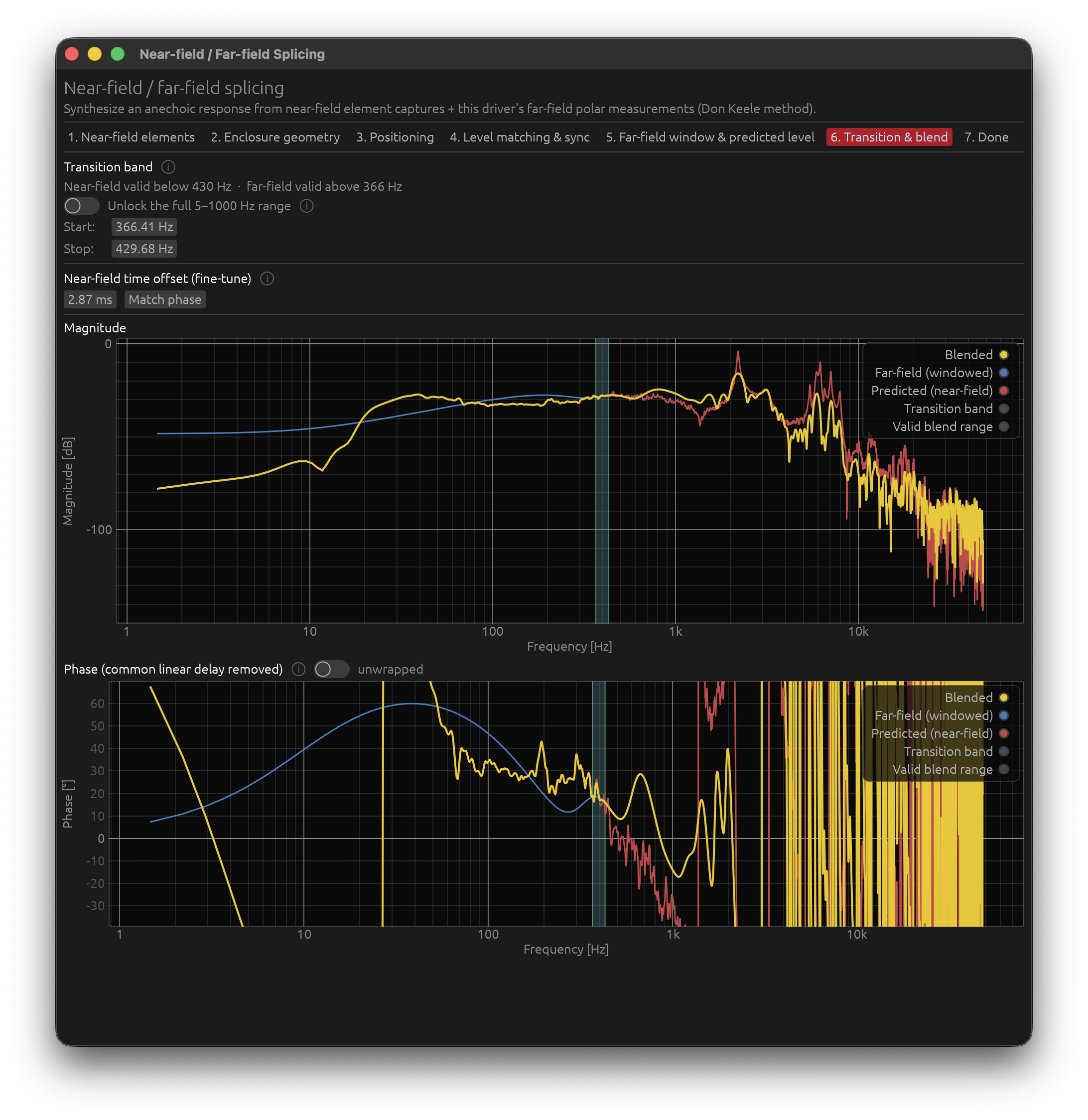
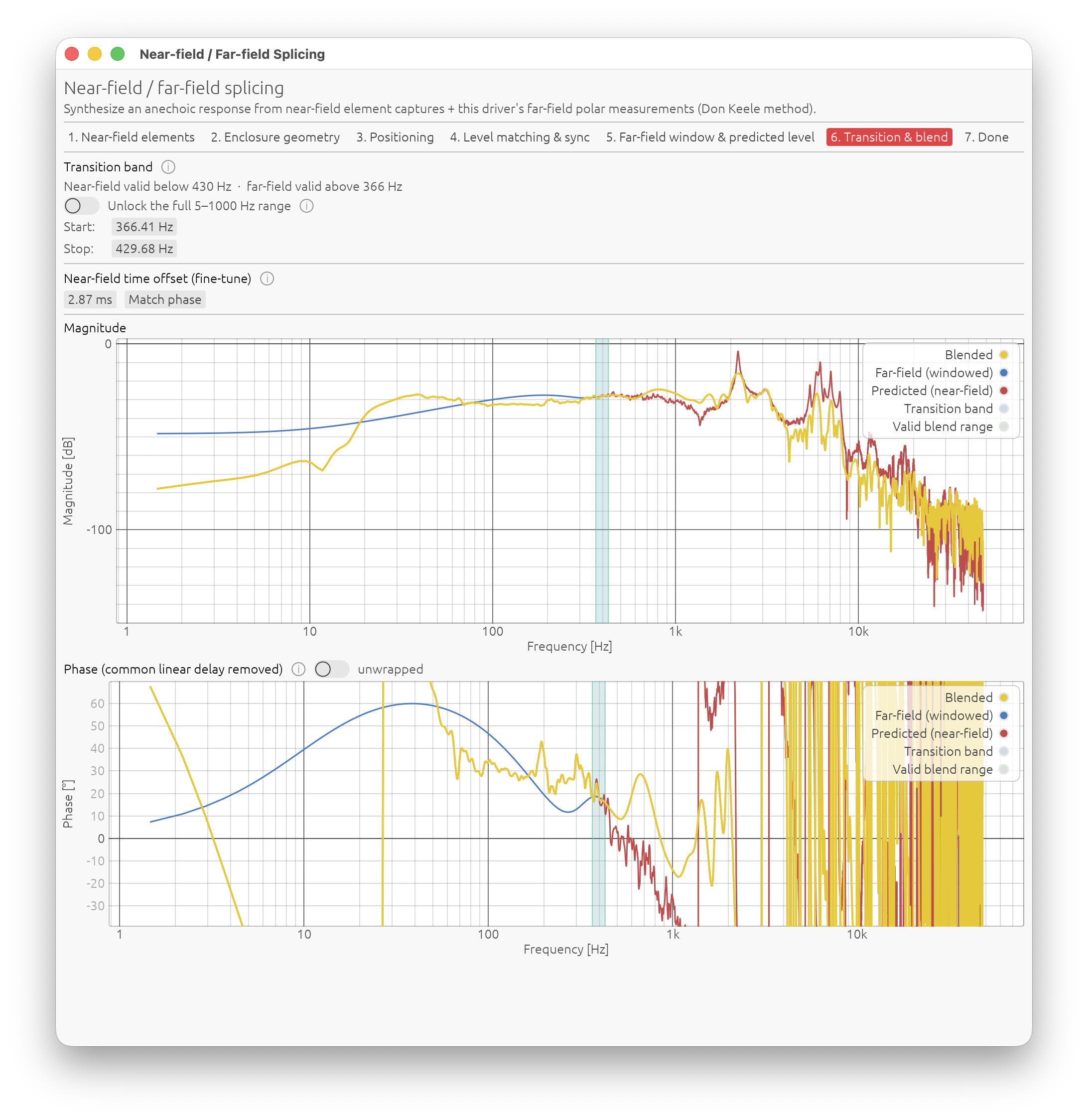
Start / Stop in Hz — where the blend hands over from the near-field prediction to the windowed far-field measurement (raised-cosine crossfade in log frequency). By default it is bounded to the valid blend range from Step 5, shaded green on both plots; the transition band itself is shaded blue inside it.
If the valid range is empty (floor above ceiling) a red message tells you why — usually lengthen the far-field window or re-measure further from the walls.
Unlocking the range
The “Unlock the full 5–1000 Hz range” toggle lifts the physical limits and lets you place Start / Stop anywhere in 5–1000 Hz, subject only to Start < Stop. The finalize step (and the auto-re-splice) then use your values as-is rather than re-clamping them.
Use it when the valid band is too narrow or empty to work with — a big woofer whose gate can’t be made long enough — and a rough splice beats none, or when you know the far-field measurement is actually cleaner than its window-length limit suggests (measured outdoors, for example).
⚠️ Past the green range the estimate degrades:
- below the far-field floor you blend in far-field bass that is contaminated by a reflection or shorter than one period;
- above the near-field ceiling you blend in near-field data that no longer matches the radiated field (reactive/evanescent field, no directivity).
Expect level and phase errors in and around the transition, worse the further the blue band spills past the green.
Advice: with the range locked, put the band as low as the far-field data allows, and keep it narrow-to-moderate. Blending low keeps as much of the real, diffraction-carrying far-field data as possible. A very wide band smears any residual level or phase mismatch across a broad range instead of confining it.
If the level still looks off here, go back to Step 5 and use Match level to far-field (next to the level offset).
Near-field time offset (fine-tune)
A ±50 ms trim on the predicted near-field response, on top of the geometric delay model. Use it to null the residual phase mismatch with the far-field measurement in the transition band.
Match phase — next to the offset — sets it automatically: it smooths out per-bin phase noise, then picks the delay that makes the predicted and far-field phase curves cross at the middle of the transition band — the geometric mid-band, where the blend is 50/50 and a phase mismatch would show up as a step in the handover. It only nulls the phase at that one point; a residual slope across the band, or a whole-turn wrap, is left for you to read off the phase plot below and nudge out by hand. It needs a far-field window and at least one captured element.
Magnitude and phase plots
Both plots show Predicted (near-field), Far-field (windowed) and Blended, with the valid blend range shaded green and the transition band shaded blue inside it.
- Magnitude — the blended curve should pass smoothly from one to the other with no step or dip.
- Phase — a shared linear-delay slope is removed from all three curves, and Predicted / Blended are shifted by a whole turn if needed to overlay Far-field, so only the residual alignment is visible. Toggle wrapped / unwrapped as you prefer (wrapped by default). Use Match phase, then tune the near-field time offset by hand until Predicted and Far-field lie on top of each other across the shaded band — that is when the blend is phase-coherent.
Step 7 — Done
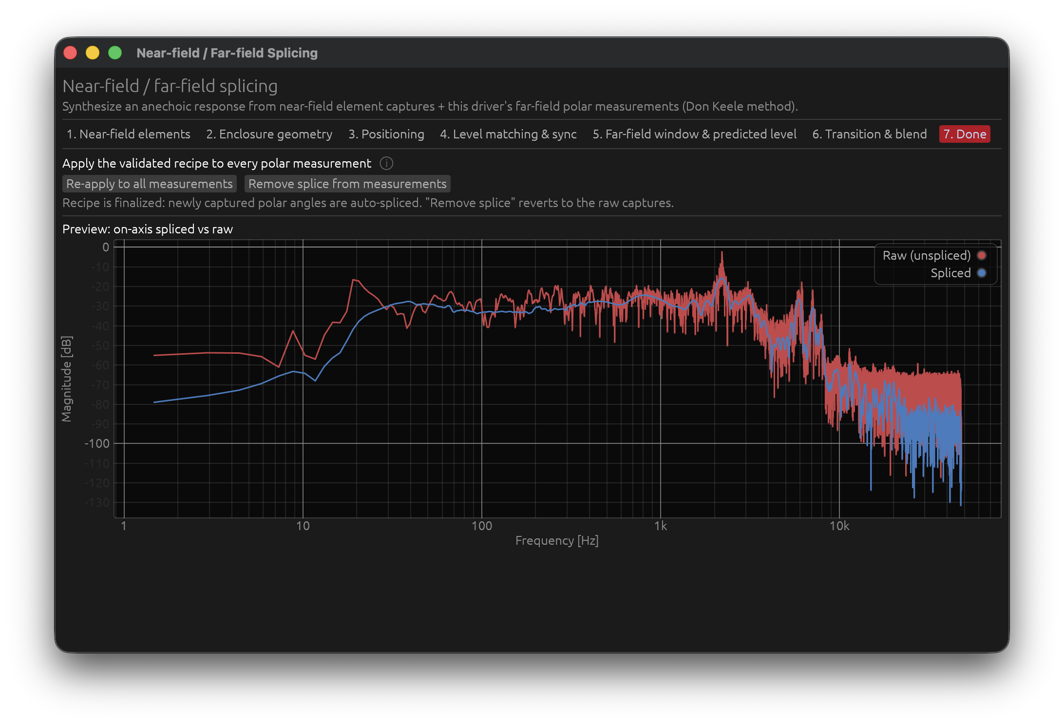
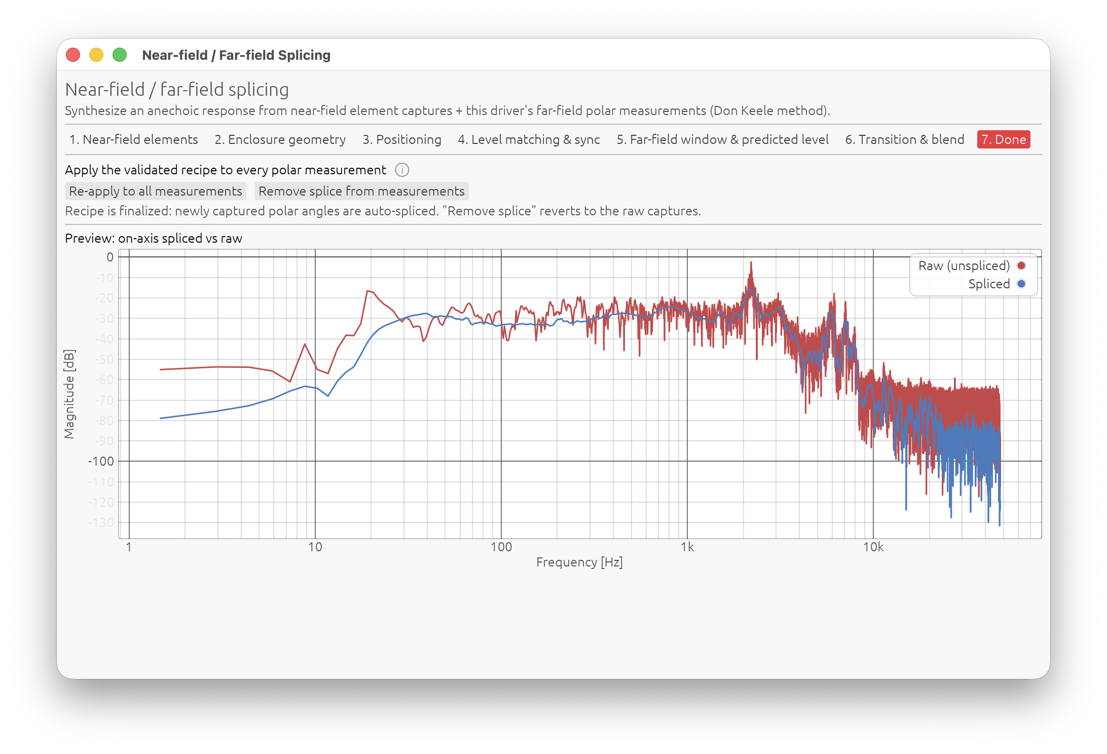
Apply the recipe to every polar measurement
Apply to all measurements takes the validated recipe and, for every stored angle:
- recomputes the geometric delay, piston directivity and edge diffraction for that angle (each polar angle sees a different diffraction path),
- blends with that angle’s own windowed far-field capture,
- reuses the far-field window, predicted level/offset and transition band from the earlier steps.
The spliced IR then replaces the raw capture everywhere in the app — response, DI, sonogram, export — for every angle that has one.
- Re-apply to all measurements — after changing anything in the recipe.
- Remove splice from measurements — reverts every angle to its raw capture.
- Preview: on-axis spliced vs raw — the before/after on axis.
Automatic re-splicing
Once the recipe is finalized, any newly captured polar angle is spliced automatically with the same recipe — you don’t have to reopen the wizard after each new measurement.
⚠️ Every polar measurement must use the same mic position and the same gain chain as the original on-axis far-field capture. The recipe reuses the mic distance / aim point from Step 3 and the far-field window and level offset from Steps 5–6 for every angle — it does not re-detect them per measurement. If you move the mic (only rotate the speaker), or change the mic preamp / interface gain between angles, the newer captures will be windowed and leveled wrong and the finalized splice will be inconsistent across angles.
How the Spliced Response Interacts with IR Windowing
A spliced IR behaves like a normal measurement. In IR Management → IR Windowing, the driver’s own time window applies on top of the spliced (anechoic) response, not on top of the raw capture.
Because the spliced response is already anechoic to the bottom of the passband, you can usually leave the driver’s IR window long or disabled for a spliced driver — its purpose (gating room reflections) has already been served by the splice.
Exporting
When you export a measurement that has a spliced version, the export dialog asks for Raw capture or Spliced (anechoic) (it defaults to spliced). Spliced exports get a _spliced marker in the filename. If the angle also has a harmonic distortion capture, Include distortion is available for either choice — it prepends the distortion tail measured at capture time to whichever main response you export, adding a _dist marker (_spliced_dist when combined with a spliced export).
Tips and Pitfalls
- Measure the mic distances and Sd carefully. They set the relative levels between elements directly. A 20 % Sd error is a ~1.5 dB level error on that element.
- Same gain chain for every near-field capture. No exceptions. There is no way to recover from a mid-session change.
- Window near-field captures loosely, far-field captures tightly. Near-field has no room to gate out; far-field must exclude the first reflection.
- Blend as low as the far-field data allows. More real far-field data = better directivity and diffraction. The near field carries no directivity information.
- A deep notch in the transition region usually means a phase mismatch — tune the near-field time offset on Step 6, don’t reach for a polarity inversion (vents and passive radiators need none; their measured near-field response already carries the anti-phase-below-tuning behaviour).
- Predicted level far from 0 dB is normal (Step 5) — the physics pre-scales by Sd.
- Re-measure away from walls if Step 6 says the room reflection prevents an overlap. No amount of tweaking fixes a far-field measurement that can’t be gated clean above the near-field ceiling.
- Large Sd + short far-field window = no valid band. A 15″ woofer’s near-field ceiling is ~350 Hz; if your far-field window only reaches down to 400 Hz there is nothing to splice. Lengthen the window.
- Use an Electric timing reference for near-field captures whenever the interface allows it. Without one — a USB measurement microphone in particular precludes it — capture-chain jitter between separately-captured elements can corrupt the sum; use Step 4’s manual sync alignment as the fallback.
Quick Reference
| Step | Purpose | Key advice |
|---|---|---|
| 1 — Near-field elements | Capture each radiator up close | Loose window, watch Sd validity ceiling |
| 2 — Enclosure geometry | Baffle size, edges | Get baffle width + edge offsets right |
| 3 — Positioning | Mic reference, element placement, room guard | Enter mic-to-wall distance |
| 4 — Level matching & sync | Relate vent/PR level to driver; fix capture jitter | Trust Sd/distance; sync only if no Electric reference |
| 5 — Far-field window & level | Gate the far-field, align levels | Window long, stop before first reflection; use Match level |
| 6 — Transition & blend | Choose the crossover band, null phase | Blend low and narrow; Match phase, then the time offset |
| 7 — Done | Apply to all angles | Re-apply after any recipe change |
Appendix: Why the Near-Field Has a High-Frequency Limit
A physicist’s / engineer’s aside. Not needed to use the wizard, but it explains where the ceiling \(f_\text{max}\) comes from and why the splice has to hand over to the far-field measurement above it.
The near-field technique in one line
The near-field method (Keele, 1974) measures the sound pressure a few millimetres in front of the diaphragm and treats it as a scaled copy of the far-field on-axis response. That works because, for an acoustically small source, the near-field pressure and the far-field pressure differ only by a frequency-independent constant.
For a rigid circular piston of radius \(a\) in an infinite baffle, the exact on-axis pressure at distance \(d\) is
$$ |p(d)| = 2 \rho c U_0 \left|\sin\left[\frac{k}{2}\left(\sqrt{d^2+a^2}-d\right)\right]\right| ,\qquad k=\frac{2\pi f}{c} $$
with \(U_0\) the piston surface velocity. Two limits:
- Near (\(d \to 0\)): \(|p_\text{near}| \approx 2 \rho c U_0 \sin(ka/2)\).
- Far (\(d = r \gg a\)): \(|p_\text{far}| \approx \rho c U_0 \dfrac{k a^2}{2r}\) — the ordinary \(p_\text{far} = \dfrac{j\omega\rho Q}{2\pi r}\) of a baffled source of volume velocity \(Q = U_0\pi a^2\).
Their ratio is
$$ \frac{|p_\text{near}|}{|p_\text{far}|} \approx \frac{2 \rho c U_0 \sin(ka/2)}{\rho c U_0 k a^2/(2r)} \xrightarrow{ka\ll 1} \frac{2r}{a} . $$
The \(\sin(ka/2)\to ka/2\) small-angle step is the whole game: it makes the rising \(\propto f\) trend cancel between numerator and denominator, leaving a constant \(2r/a\). Measure near, multiply by that constant, and you have the far-field magnitude response — as long as \(ka \lesssim 1\). LinFIR uses
$$ f_\text{max} = \frac{c}{2\pi a} = \frac{c}{2\sqrt{\pi S_d}} \qquad\Longleftrightarrow\qquad ka = 1 . $$
Above it, \(\sin(ka/2)\) leaves its linear region, the near-field pressure grows its own interference ripple, and the far field starts developing directivity — so the ratio is no longer a constant and the method breaks.
The reactive (evanescent) field
Why is a small source “special”? Decompose the diaphragm’s surface velocity into spatial Fourier components with transverse wavenumber \(k_\parallel\). Each component launches a plane wave at angle \(\sin\theta = k_\parallel/k\):
- \(k_\parallel < k\): a real angle exists — the component radiates.
- \(k_\parallel > k\): no real angle — the field is evanescent, decaying away from the surface as \(e^{-\gamma z}\) with \(\gamma = \sqrt{k_\parallel^{2}-k^{2}}\).
A feature of transverse size \(\ell\) carries \(k_\parallel \sim \pi/\ell\), so its evanescent field is gone within \(z \sim \ell\). The edge of the piston — where the velocity jumps from \(U_0\) to \(0\) — and any cone break-up inject large \(k_\parallel\); all of that is evanescent unless the feature is bigger than a wavelength.
When \(ka \ll 1\) the whole radiator is smaller than \(\lambda\): essentially none of its spatial content satisfies \(k_\parallel < k\), so the field right at the surface is dominated by the reactive/evanescent part — air being pushed sideways between regions of the cone and springing back, storing kinetic energy without radiating it. This shows up in the piston’s radiation impedance \(Z_\text{rad} = \rho c[R_1(2ka) + j X_1(2ka)]\):
$$ R_1(2ka) \approx \frac{(ka)^2}{2}, \qquad X_1(2ka) \approx \frac{8 ka}{3\pi}, \qquad \frac{X_1}{R_1} \approx \frac{16}{3\pi ka}. $$
For \(ka \ll 1\) the reactance swamps the resistance: the source is a poor radiator that mostly sloshes air around locally. The two become comparable — the radiation-impedance “knee” — at \(ka\) of order 1, the same place the near-field validity ends.
Crucially, in that reactive regime the on-axis near-field pressure is still the simple, position-tolerant quantity above (\(\propto U_0 \sin(ka/2)\)); the messy evanescent structure lives off-axis and in the tangential field. That is exactly why the trick works — and why it stops working once real radiation, with its own propagating interference, takes over.
Connection to directivity
Directivity is the angular shape of the radiating (\(k_\parallel < k\)) part of the field, seen in the far zone. Track it against \(ka\):
- \(ka \lesssim 1\): only the lowest-\(k_\parallel\) sliver of the source’s spectrum radiates, and it looks like a monopole — the speaker is omnidirectional.
- \(ka \sim 1\text{-}3\): more of the spectrum crosses below \(k\); the pattern starts to narrow.
- \(ka \gg 1\): the pattern locks into the piston beaming law \(D(\theta) = \dfrac{2 J_1(ka\sin\theta)}{ka\sin\theta}\).
So the near-field measurement is trustworthy precisely in the band where the loudspeaker has essentially no directivity. The onset of directivity and the breakdown of the near-field proxy are the same event, both governed by \(ka \approx 1\): directivity is the structure of the radiated field, and that structure only becomes well defined once the evanescent field — which decays exponentially with distance, \(e^{-\gamma z}\), over a few source dimensions — has faded relative to the propagating field.
Why the splice is built the way it is
- Below \(f_\text{max}\): the speaker is omnidirectional and the near-field pressure is a clean, scaled copy of the far-field response. The splice takes the near-field magnitude and phase here — there is no directivity to lose.
- Above \(f_\text{max}\): the near-field reading is corrupted by its own interference and the speaker is starting to beam. The splice must use the real far-field measurement, which carries the diffraction and directivity the near field never had.
- The transition band lives in the overlap where both are still acceptable. The wizard caps it at \(f_\text{max}\) (and at the far-field floor) for that reason; the unlock toggle lets you override it when no valid overlap exists, at a known cost to accuracy.