IR Management
The IR (Impulse Response) Management window provides comprehensive tools for obtaining, processing, and managing impulse responses for each driver or measurement position in your system.
Accessing IR Management
Loudspeaker Design Mode:
- To open: Driver → Manage IR
- Purpose: Import, capture, and process driver impulse responses at multiple angles
Room Calibration Mode:
- To open: Measurements → Manage IR
- Purpose: Capture IR at a given in room position
Driver/Measurement Name
Manually enter a descriptive name for the impulse response.
- Label: “Driver Name” (Loudspeaker Design) or “Measurement Name” (Room Calibration)
- Purpose: Identify IRs in project and exports
- Persistence: Names are saved with the project
- Optional: Empty names default to “Driver X” or “Measurement X”
- Best practice: Use descriptive names like “Woofer_Left”, “Tweeter_RefXYZ”, “Position_Center”
Capturing IR
Button: 🎤 Measure
Triggers a measurement sweep with the configured parameters to capture the impulse response.
Features:
- Exponential sine sweep generation with configurable parameters
- Automatic harmonic distortion analysis (THD)
- Timing reference support for multi-driver measurements
For complete documentation on sweep parameters, driver protection, measurement workflow, and best practices, see Sweep Measurements.
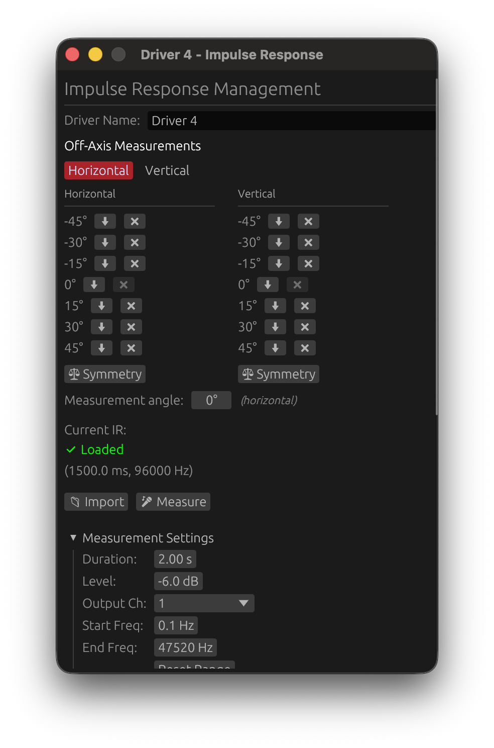
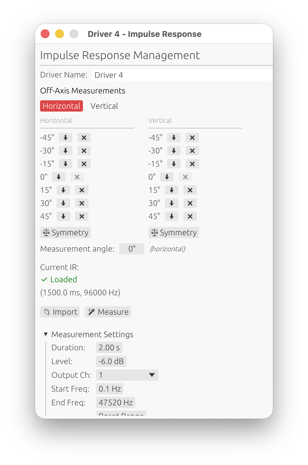
Off-Axis Measurements 🔒
Available in: Loudspeaker Design mode only License required: Valid LinFIR license needed for off-axis measurements
Overview
Off-axis measurements enable directivity analysis by capturing impulse responses at different horizontal and vertical angles. These measurements are essential for understanding speaker radiation patterns and optimizing crossover design for consistent off-axis response.
Measurement Organization
Measurements are displayed in two columns:
-
Horizontal column: Measurements with vertical angle = 0°, varying horizontal angle
- Example: -90°, -60°, -30°, 0°, +30°, +60°, +90°
-
Vertical column: Measurements with horizontal angle = 0°, varying vertical angle
- Example: -60°, -40°, -20°, 0°, +20°, +40°, +60°
On-axis reference: The (0°, 0°) measurement appears in both columns.
Axis Selection
Before importing or capturing an off-axis measurement, select the measurement axis:
- Horizontal button: Measurements along horizontal axis (left/right)
- Vertical button: Measurements along vertical axis (up/down)
The selected axis determines whether the angle applies to horizontal or vertical position.
Measurement Angle
Field: “Measurement angle” Range: -180° to +180° Indicates: Angle for next import or capture operation
How it works:
- If Horizontal axis selected: angle applies to horizontal position (vertical = 0°)
- If Vertical axis selected: angle applies to vertical position (horizontal = 0°)
- The field shows which axis is active: “(horizontal)” or “(vertical)”
Restrictions:
- Disabled until on-axis (0°, 0°) measurement exists
- Requires valid LinFIR license
- Must import on-axis measurement first before adding off-axis angles
Per-Measurement Actions
Each measurement in the table has two action buttons:
Export Button (⬇)
Click to export this specific measurement:
- Opens export format dialog
- Choose WAV or TXT format
- Option to include distortion metadata
- File is saved with angle suffix (e.g.,
Driver1_v0h30.wav,Driver1_v-15h0.wav)
Delete Button (❌)
Remove a measurement from the driver:
- Off-axis measurements: Can be deleted freely
- On-axis (0°, 0°) measurement: Can only be deleted if all off-axis measurements are removed first
- This restriction exists because the on-axis measurement serves as the reference for all filter calculations
Tooltip guidance:
- Enabled: “Delete measurement”
- Disabled: “Delete all off-axis measurements first”
Export All Button
Button: ⬇ Export All Location: Above “Measurement angle” field Purpose: Export all measurements in a single operation
How it works:
- Click “⬇ Export All”
- Select output directory in file dialog
- All measurements are exported as WAV files
- Files use consistent naming:
DriverName_v{vertical}h{horizontal}.wav
File naming examples:
- On-axis:
Driver 1_v0h0.wav - Horizontal +30°:
Driver 1_v0h30.wav - Vertical -15°:
Driver 1_v-15h0.wav - Horizontal -45°:
Driver 1_v0h-45.wav
Format:
- All files exported as WAV (32-bit float, mono)
- Sample rate matches original measurement or importation sample rate
- Distortion metadata option applies to all files
- No individual format selection (always WAV)
Benefits:
- Fast export of complete measurement sets
- Consistent naming for re-import or external processing
- Files can be re-imported via batch import with automatic angle detection
Use cases:
- Archiving complete measurement sets
- Sharing measurements with collaborators
- Processing measurements in external tools (FIR Designer, Matlab, etc.)
Symmetry Tool
Button: ⚖ Symmetry Location: Below each column Purpose: Automatically duplicate measurements to opposite angles
How it works:
- Horizontal Symmetry: If you have +30°, creates -30° by mirroring the measurement
- Vertical Symmetry: If you have +20°, creates -20° by mirroring the measurement
Use case: Save measurement time by capturing one side and mirroring to the other side, assuming the speaker has symmetric radiation.
Workflow for Off-Axis Measurements
- Import or capture on-axis measurement (0°, 0°) first
- Select axis (Horizontal or Vertical)
- Set measurement angle (e.g., +30°)
- Import file or capture measurement
- Repeat for additional angles
- Use Symmetry tool to fill opposite angles (optional)
- Analyze directivity patterns in main application graphs
🔄 Automated workflow: If you have a motorized turntable (Pololu Tic or GRBL/Arduino), use the ▶ Scan button to rotate and measure all angles automatically. See Auto-Scan with a Rotation Table and Rotation Table Settings.
Import from File
Load impulse responses from external files.
LinFIR works internally with impulse responses (IRs). All imported files are ultimately converted to an IR before being used for filter design. Two import paths exist:
- Direct IR formats (WAV, TXT, TMD): Files already contain time-domain impulse response samples. They are resampled to the project sample rate and loaded directly.
- Frequency-domain format (FRD): Files contain frequency response data (magnitude + phase). LinFIR reconstructs an impulse response via the FRD to IR Converter window before proceeding.
Supported Formats
WAV Files
- Channels: Mono or stereo (left channel used for stereo files)
- Bit depth: 16-bit, 24-bit, or 32-bit PCM
- Automatic resampling: The IR is resampled to match the project sample rate for processing. The original samples are preserved internally at their native rate, so changing the project sample rate later does not cause quality loss from successive resamplings. This is handled transparently in the background.
With distortion metadata:
- If WAV contains custom ‘dist’ chunk (exported from LinFIR with “Include dist.” option)
- Enables THD (Total Harmonic Distortion) computation
Without distortion metadata:
- Standard WAV import
- Only practical/cropped IR available
- THD computation not available
TXT Files
Plain text files containing impulse response samples, one value per line or space/comma-separated. LinFIR auto-detects this format.
Note: .txt files containing FRD-formatted data (3 columns: frequency, magnitude, phase) are automatically detected and processed as FRD files (see FRD Files section below).
TMD Files
MATAA (Mat’s Audio Analyzer) time-domain data format. Each line encodes a sample with its timestamp, allowing the sample rate to be derived from the data itself.
- Format: Two-column text file (time in seconds, amplitude)
- Comments: Lines starting with
*are metadata/comments - Sample rate: Inferred from the time intervals between samples. If the result is within 1% of a standard rate (44.1, 48, 88.2, 96, 176.4, 192, 384 kHz, etc.), LinFIR snaps to that exact rate to correct for the systematic sample rate error introduced by limited timestamp precision.
- Timestamp precision: Timestamps must have enough decimal places for accurate sample rate inference (e.g. 9 digits for 96 kHz). Insufficient precision can produce a slightly off sample rate that will still be corrected if it falls within the 1% snapping tolerance.
- Precision: Full floating-point precision (no bit-depth limitations)
Example TMD file:
* TMD data written by MATAA
* Measurement description
0.000000000	0.000000
0.000020833	0.125000
0.000041667	0.850000
...
CLIO Files
Time-domain impulse response exports from CLIO (Audiomatica) measurement software. These are plain .txt files with three columns.
- Format: Text file with a header row followed by data rows
- Column 1 —
Time[s]: sample timestamp in seconds - Column 2 —
Real[Pa]: signal amplitude (used as the IR) - Column 3 —
Imag[Pa]: imaginary part (ignored by LinFIR)
- Column 1 —
- Header line: the first non-empty line must start with
Time(case-insensitive) - Sample rate: inferred from the time intervals between samples, then snapped to the nearest standard rate within 1% tolerance (same algorithm as TMD)
- Precision: full floating-point precision
Example CLIO file:
Time[s]         Real[Pa]        Imag[Pa]
0.000000E+00    -4.790139E-03   -4.583853E-10
2.083333E-05     4.526122E-03   -8.076313E-10
4.166667E-05     3.454284E-04    1.007265E-10
...
FRD Files
Frequency response data files (commonly exported by REW, VituixCAD, or provided by manufacturers). These files do not contain an impulse response directly—LinFIR reconstructs one via the FRD to IR Converter window (see dedicated section below).
Format:
- 3 columns per line: Frequency (Hz), Magnitude (dB), Phase (degrees)
- Text-based, space or tab delimited
- Can use either
.frdextension or.txtextension (auto-detected)
Processing:
- Automatic interpolation to required frequency points using PCHIP (Piecewise Cubic Hermite Interpolating Polynomial)
- Configurable magnitude extrapolation for DC and high-frequency regions
- Phase handling with group delay compensation
Extrapolation Modes:
When importing FRD files, LinFIR opens the FRD to IR Converter window with the following extrapolation controls:
-
DC Extrapolation: Controls how magnitude is extended below the lowest measured frequency
- Constant: Flat extrapolation (holds the lowest measured value)
- Roll-off: Applies a 12 dB/octave high-pass roll-off for realistic loudspeaker behavior
- Default: Roll-off
-
High Frequency Extrapolation: Controls how magnitude is extended above the highest measured frequency toward Nyquist
- Constant: Flat extrapolation (holds the highest measured value)
- Roll-off: Applies a 12 dB/octave low-pass roll-off, automatically compensates for upward slopes
- Default: Constant
Benefits of Roll-off mode:
- More realistic impulse responses from incomplete FRD data
- DC roll-off mimics natural loudspeaker low-frequency limitations
- HF roll-off prevents artifacts from measurements that don’t extend to Nyquist
- Adaptive: compensates for incorrect slope trends in measured data
Important notes:
- FRD files are sparse (often logarithmically spaced frequency points)
- Requires complex interpolation, potentially introducing artifacts
- Generally do not contain the time of flight required to properly time align drivers
- Recommendation: Prefer importing impulse responses (WAV) whenever possible
Automatic Noise Truncation
Once an impulse response has been imported or reconstructed (from any format), LinFIR automatically truncates it to optimize file length and processing performance. This is an internal post-processing step applied uniformly to all IR data before it is stored in the project.
Truncation Algorithm:
- Peak detection: Locates the main impulse peak (maximum absolute value in the IR)
- 5-second limit: Truncates the IR to 5 seconds maximum after the peak
- Corresponds to approximately 1.7 km acoustic distance
- Sufficient for capturing full decay in most practical scenarios
- Noise threshold: Removes trailing samples below 0.1% of peak amplitude
- Adaptive threshold based on the actual signal level
- Eliminates noise floor without affecting useful signal
- Minimum duration: Always preserves at least 1.0 seconds of the IR
- Ensures sufficient data for low-frequency analysis
Benefits:
- Reduces processing load for FFT operations and convolutions
- Decreases file sizes for project saving and export
- Removes unnecessary noise floor that doesn’t contribute to filter design
What gets removed:
- Excessive silence beyond 5 seconds after the main impulse
- Noise floor below the 0.1% threshold (≈ -60 dB relative to peak)
- Applies to both anechoic and in-room measurements
What is preserved:
- The complete main impulse and initial decay
- At least 1.0 seconds of IR data regardless of noise level
- All frequency content relevant for crossover design
- Sufficient time-domain information for phase analysis
Impulse Response Timing Requirements
Peak delay limit: LinFIR rejects impulse responses where the main peak is located more than 200 ms after the start of the file.
Why this limit exists:
LinFIR performs extensive signal processing operations—FFT transformations, convolutions, resampling, and real-time filter preview—that must remain responsive. These operations scale with impulse response length, and excessive zero padding before the actual signal significantly impacts performance without adding useful information.
Physical context:
A 200 ms delay corresponds to approximately 68 meters of acoustic travel distance. In practical loudspeaker measurement and room calibration scenarios, such excessive delays indicate that no timing reference method was used during capture (loopback trigger, electrical reference, or pre-alignment in the measurement software).
Impact on workflow:
Without proper timing reference, relative time alignment between drivers becomes unreliable, as the arbitrary delays vary unpredictably between measurements. This compromises crossover phase coherence and summation accuracy—core functions of LinFIR.
Best practice:
When capturing impulse responses, use measurement software that provides:
- Loopback triggering (audio interface output → input reference)
- Electrical reference triggering (synchronized start)
- Pre-alignment features that position the IR peak near the beginning of the recording
These methods ensure minimal file length while preserving the precise time-of-flight information needed for accurate driver alignment and filter design.
If your measurement contains a valid signal buried in initial silence, pre-process the file to remove leading zeros before importing into LinFIR.
Import Workflow
- Click “📁 Import” button
- Select WAV, TXT or FRD file
- File is automatically detected and processed:
- WAV: Resampled to project sample rate, metadata extracted
- TXT (impulse samples): Either auto-imported (with metadata) or user prompted for sample rate
- TXT/FRD (frequency data): Opens FRD to IR Converter window
- IR appears in impulse response graph
- Manually enter IR name in text field
- Apply windowing if necessary (see Time Windowing section)
Special case for FRD files: When importing .frd or FRD-formatted .txt files, the FRD to IR Converter window opens automatically. See the dedicated section below for details.
⚠️ Display Mode Check: If the imported impulse response does not appear in the graphs, verify that Drivers/Measurements display mode is selected in the graph toolbar (not FIR, IIR, or FIR+IIR modes which only show filter responses). The graph title and legend clearly indicate which mode is active.
Batch Import of Multiple Measurements
Available in: Loudspeaker Design mode (off-axis measurements) License required: Valid LinFIR license needed for off-axis measurements
Overview
Batch import enables importing multiple measurement files simultaneously with automatic angle detection from filenames. This significantly speeds up the workflow when importing multi-angle measurement sets from tools like VituixCAD, ARTA, or REW.
Filename Angle Parsing
LinFIR automatically detects measurement angles from filenames using conventions from other measurement software.
Important: Angle patterns must be at the end of the filename (before extension). If the axis marker (h/v) has a prefix format (like h30), it must not be preceded by a letter. This prevents false detection in cases like “Driverh30” while allowing “SIG270-4h30” or “Driver 2_h30”.
Format with single axis specification (H = Horizontal, V = Vertical):
H30,h30,H-20→ Horizontal axis, angles: +30°, +30°, -20°V15,v15,V-45→ Vertical axis, angles: +15°, +15°, -45°30H,30h,-20H→ Horizontal axis, angles: +30°, +30°, -20°15V,15v,-45V→ Vertical axis, angles: +15°, +15°, -45°
Format without axis (@ marker):
@30,@-20,Tweeter@15→ Angle detected, axis must be specified by user- When files use @ notation, a dialog prompts you to select Horizontal or Vertical axis
MF 2D format (both H and V in filename):
v0h30,V0H30,v000h030→ Horizontal +30° (horizontal plane: V=0)v30h0,V30H0,v030h000→ Vertical +30° (vertical plane: H=0)h30v0,H30V0,h030v000→ Horizontal +30° (order-independent)h0v30,H0V30,h00v030→ Vertical +30° (order-independent)v0h0,V0H0,v000h000→ On-axis (0°, 0°)v30h50→ Rejected (out-of-plane measurement)
Note: Leading zeros are supported (e.g., 030 = 30)
Note on MF 2D format: Only measurements in a plane are accepted (one angle must be 0). Files with both H and V non-zero are ignored as they represent oblique measurements that can’t be represented in LinFIR’s horizontal/vertical coordinate system. The order of h/v doesn’t matter.
Examples of valid filenames:
Tweeter_h0.wav→ On-axis (0°, 0°)Tweeter_h30.wav→ Horizontal +30°Tweeter_v-20.frd→ Vertical -20°Woofer@15.txt→ Angle +15° (user selects axis)measurement_30h.wav→ Horizontal +30°Left_-45v.frd→ Vertical -45°Driver_v0h45.frd→ Horizontal +45° (MF 2D format)Tweeter_v20h0.txt→ Vertical +20° (MF 2D format)SIG270-4h30.frd→ Horizontal +30° (number before axis letter is OK)SIG270-4v0h30.frd→ Horizontal +30° (MF 2D with number prefix)
Examples of rejected filenames:
Driverh30.wav→ Rejected (letter “r” directly before “h”)Testh30v0.frd→ Rejected (letter “t” directly before “h”)
Files without angle markers:
- Imported as on-axis (0°, 0°) measurement
- You can still manually set the angle before importing if needed
Batch Import Workflow
1. Multi-File Selection
- Click “📁 Import” button
- Select multiple files in the file dialog (Ctrl+Click or Shift+Click)
- Click Open
2. Automatic Processing
LinFIR automatically analyzes all selected files:
If all files have explicit axis (H/V in filename):
- Files are processed immediately
- Each file imported at the angle specified in its filename
- No user interaction needed
If files use @ notation (ambiguous axis):
- Axis Selection Dialog appears
- Select either Horizontal or Vertical axis
- Click Continue
- Selected axis applies to all @ files in the batch
3. FRD Converter Integration
If the batch includes FRD files:
- LinFIR opens the FRD Converter for the on-axis FRD file (if present)
- Configure conversion parameters (sample rate, delay, extrapolation modes)
- Click “Use This Impulse Response”
- All remaining FRD files automatically use the same parameters
- No need to configure each file individually
How it works:
- Parameters are configured using the on-axis measurement (0°, 0°)
- Same delay and extrapolation settings applied to all off-axis FRD files
- Ensures consistent conversion across the measurement set
⚠️ Important Limitation - Missing Relative Time Delays:
FRD files contain frequency response data only (magnitude and phase) without encoding the relative time delays between different measurement angles. When importing multiple FRD files at different angles, all files use the same delay parameter configured on the on-axis measurement.
Why this matters for off-axis measurements:
In real loudspeakers, off-axis measurements have different acoustic path lengths and interference patterns compared to on-axis:
- Sound from tweeter and woofer arrives at different relative times depending on measurement angle
- These time differences create frequency-dependent interference (comb filtering)
- Proper time alignment between drivers varies with angle
Consequence:
- Batch-imported FRD files will have identical relative timing at all angles
- Phase relationships between drivers won’t reflect actual acoustic behavior
- Directivity analysis and crossover optimization will be inaccurate
- Simulated off-axis response won’t match real-world interference patterns
Recommendation:
- Prefer WAV impulse response files for multi-angle measurements whenever possible
- WAV files preserve the actual time-of-flight at each angle
- Only use FRD batch import for preliminary analysis or when WAV files aren’t available
- If using FRD files, be aware that off-axis crossover behavior won’t be accurately modeled
Valid use cases for batch FRD import:
- Quick magnitude response comparison across angles
- Preliminary directivity visualization
- Single-driver systems where relative timing isn’t critical
- When no impulse response measurements are available
Practical Example
Scenario: You have a set of horizontal measurements exported from REW:
Tweeter_h0.frd
Tweeter_h15.frd
Tweeter_h30.frd
Tweeter_h45.frd
Tweeter_h60.frd
Workflow:
- Select all 5 files in file dialog
- FRD Converter opens for
Tweeter_H0.frd(on-axis) - Set sample rate to 96000 Hz, delay to 5 ms
- Choose DC extrapolation: Roll-off
- Click “Use This Impulse Response”
- Files
H15,H30,H45,H60automatically converted with same settings - All 5 measurements appear in the horizontal column
Result:
- All angles have same delay (5 ms) configured on on-axis measurement
- ⚠️ Relative time-of-flight differences between angles are lost
- For accurate crossover modeling, prefer WAV impulse response files
Limitations
- Batch import only works with files having consistent format (all WAV, all FRD, or mixed)
- Files must follow supported angle naming conventions
- On-axis measurement (0°, 0°) should be included when importing FRD files for optimal parameter configuration
- If mixing WAV and FRD formats, FRD files must include on-axis or parameters will use defaults
- FRD files don’t preserve relative time delays between angles—prefer WAV files for multi-angle measurements
Tips
Consistent naming convention:
- Use descriptive base names:
Tweeter_h30.wavinstead of justh30.wav - Include driver name in filename for easier identification
- Use lowercase h/v for consistency with LinFIR exports
- MF 2D format is order-independent:
v0h30=h30v0
Large measurement sets:
- Import horizontal and vertical measurements separately if you have both
- Use Symmetry tool after batch import to fill missing opposite angles
- Verify measurement table after import to ensure correct angle assignment
FRD files:
- ⚠️ Not recommended for off-axis measurements (missing relative time delays)
- Always include on-axis (H0 or V0) measurement in batch for parameter reference
- Configure extrapolation modes carefully for first file—settings propagate to all
- Verify impulse response quality after batch conversion
- Consider this a preliminary workflow—prefer WAV files for accurate directivity analysis
Recommended format priority:
- WAV files: Best option—preserves all timing information
- TXT with metadata: Acceptable if exported from LinFIR
- FRD files: Only for magnitude analysis—timing not preserved
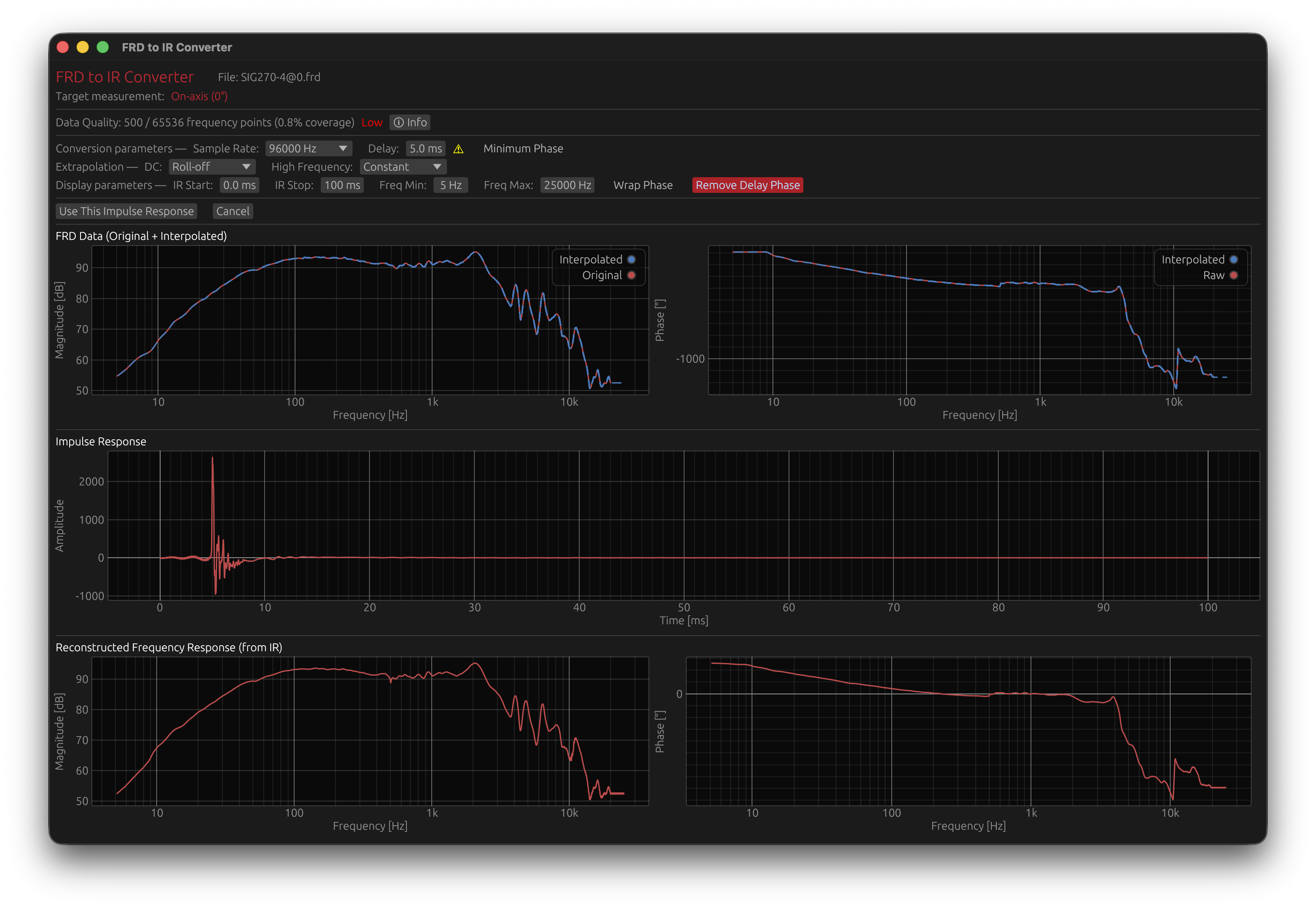
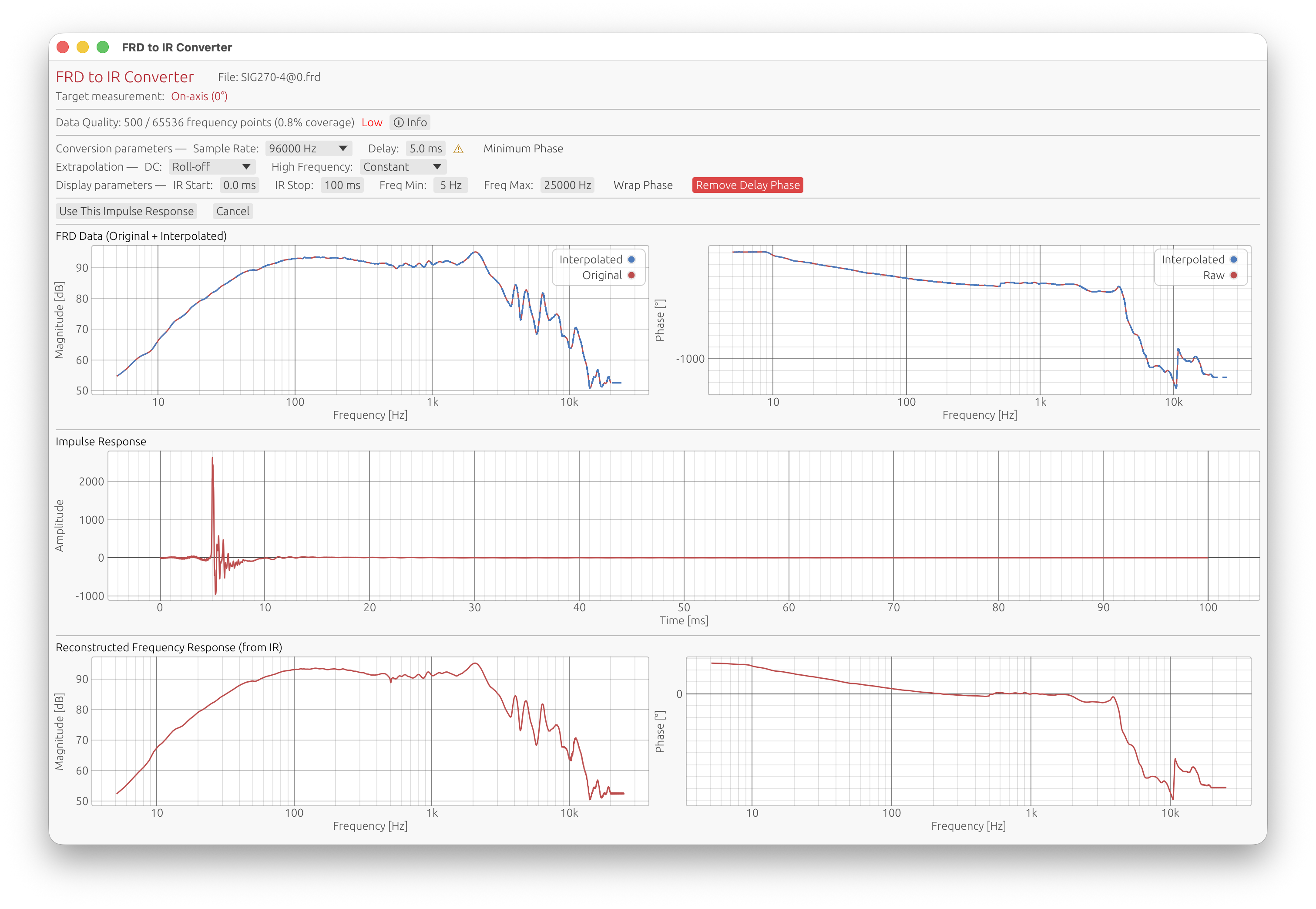
FRD to IR Converter
When importing FRD files, LinFIR opens a dedicated conversion window with advanced tools for interpolation, visualization, and quality assessment.
Overview
The FRD to IR Converter transforms sparse frequency-domain data into time-domain impulse responses using sophisticated interpolation and extrapolation techniques. It provides real-time visualization and quality metrics to help you assess the conversion quality.
Conversion Parameters
Sample Rate
Options: 44.1 kHz, 48 kHz, 88.2 kHz, 96 kHz, 176.4 kHz, 192 kHz Default: 96 kHz
Target sampling frequency for the resulting impulse response.
Considerations:
- Higher sample rates provide better frequency resolution
- Must match or exceed your project’s sample rate
- FRD data is interpolated to fill all frequency bins from DC up to Nyquist
Delay Compensation
Range: 0.0 to 100.0 ms Default: 5.0 ms
Time offset applied to the impulse response to allow for pre-ringing visualization and processing.
Purpose:
- Provides time buffer before the main impulse
- Essential when FRD data contains non-minimum phase characteristics
- Allows visualization of pre-ringing artifacts
Warning indicator: If pre-ringing duration exceeds the delay setting, a warning appears suggesting either:
- Increase delay to accommodate pre-ringing
- Enable Minimum Phase transformation
Minimum Phase Transformation
Default: Disabled
Applies Hilbert transform to convert the impulse response to minimum phase, eliminating all pre-ringing.
When to use:
- FRD data shows significant pre-ringing (> 5% energy before peak)
- Phase data is corrupted, smoothed, or contains wrapping errors
- You need a causal, physically realizable impulse response
- Time-domain alignment is critical
Effects:
- Removes all energy before the main peak
- Preserves magnitude response
- Changes phase response to minimum phase equivalent
- Results in a causal system (no pre-ringing)
Note: Pre-ringing in FRD-derived impulses is often an artifact of measurement or file creation, not a physical characteristic of the device.
DC Extrapolation
Modes: Constant, Roll-off Default: Roll-off
Controls how magnitude is extended below the lowest measured frequency toward DC (0 Hz).
Constant mode:
- Flat extrapolation using the lowest measured value
- Use when FRD data already reaches very low frequencies
Roll-off mode (recommended):
- Applies 12 dB/octave high-pass characteristic
- Mimics natural loudspeaker low-frequency roll-off
- More physically realistic for incomplete low-frequency data
High Frequency Extrapolation
Modes: Constant, Roll-off Default: Constant
Controls how magnitude is extended above the highest measured frequency toward Nyquist.
Constant mode (recommended):
- Flat extrapolation using the highest measured value
- Maintains adequate signal level to Nyquist
- Minimizes noise amplification
Roll-off mode:
- Applies 12 dB/octave low-pass characteristic
- Automatically compensates for upward slope trends
- Use when FRD data shows unrealistic high-frequency behavior
Driver Offset Compensation
The FRD to IR Converter provides Driver Offset controls to compensate for the physical displacement of the driver relative to the reference point (typically the front baffle center or another driver).
Parameters:
- X (Horizontal): Driver offset in the horizontal direction, in millimeters
- Y (Vertical): Driver offset in the vertical direction, in millimeters
- Located below the Extrapolation controls in the converter window
Coordinate System and Geometry:
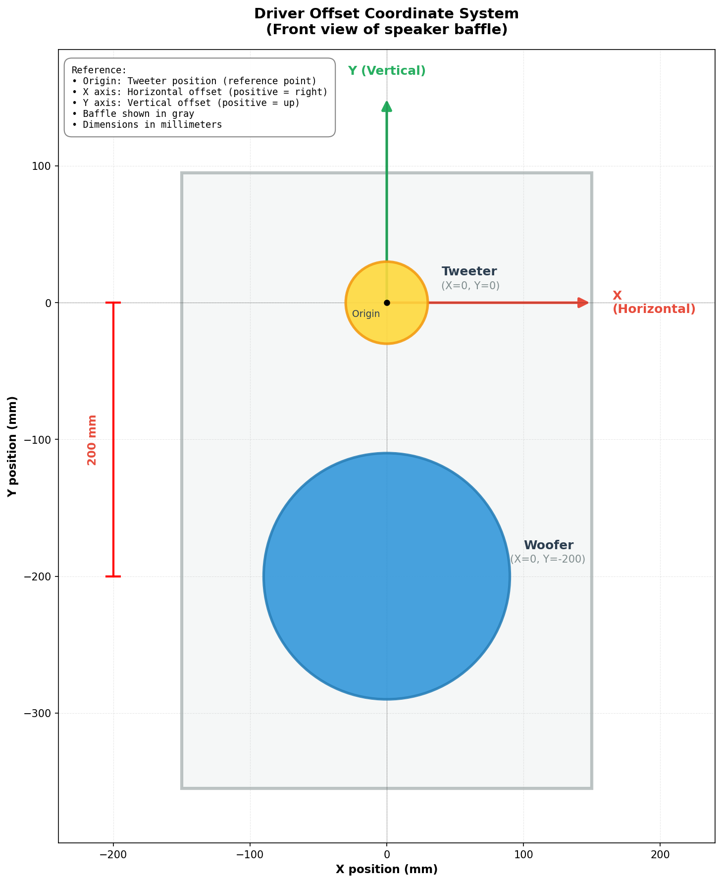
Reference Point (Origin):
The reference point (X=0, Y=0) represents the desired acoustic axis of the loudspeaker system. In the diagram example:
- The tweeter is positioned at the origin (0, 0) — it defines the acoustic axis
- The woofer is offset by -200 mm vertically (0, -200)
Note for designers: The choice of origin is not necessarily the center of a driver — it’s an engineering decision. You could choose:
- The acoustic center of a specific driver (as shown in the example)
- A point between drivers (e.g., midway between tweeter and woofer)
- Any other reference point that makes sense for your design goals
What matters is consistency: all driver offsets are measured relative to this chosen origin.
Important: For off-axis measurements, only a driver with offset (woofer in the example) will have geometric delay applied. A driver at the origin (tweeter in the example) has no delay added or subtracted for off-axis angles — it remains the reference. This delay difference is then used to calculate interference patterns between drivers at off-axis angles.
How it works:
The driver offset introduces an additional geometric delay for off-axis measurements, calculated using the far-field approximation with Euclidean distance:
$$\Delta t = \frac{\sqrt{(x \cdot \sin\theta)^2 + (y \cdot \sin\varphi)^2}}{c}$$
Where:
- \(x\) = horizontal driver offset (mm)
- \(y\) = vertical driver offset (mm)
- \(\theta\) = horizontal measurement angle (degrees)
- \(\varphi\) = vertical measurement angle (degrees)
- \(c\) = speed of sound ≈ 343,000 mm/s
In practice (measurements in a single plane):
Since LinFIR only supports measurements in the horizontal plane (\(\theta \neq 0\), \(\varphi = 0\)) or vertical plane (\(\theta = 0\), \(\varphi \neq 0\)), the formula simplifies:
- Horizontal plane: \(\Delta t = \frac{x \cdot \sin\theta}{c}\) (only x offset matters)
- Vertical plane: \(\Delta t = \frac{y \cdot \sin\varphi}{c}\) (only y offset matters)
The Euclidean formula is used in the code to be mathematically correct and future-proof should oblique measurements be supported.
This geometric delay is added to the user-configured delay before converting the FRD data to an impulse response.
Example:
- Tweeter at origin (0, 0): no geometric delay applied at any angle
- Woofer offset: X = 0 mm, Y = -200 mm
- Measurement at vertical -30° (30° below axis)
- Geometric delay for woofer: \(200 \times \sin(30°)/343000 \approx 0.291\) ms
- This delay difference creates the correct interference pattern between tweeter and woofer at -30°
Purpose and Far-Field Approximation:
⚠️ Purpose: Driver offsets are used to predict far-field interference patterns between drivers when the listener is in the far field (listening distance >> driver spacing).
Key insight: Since typical FRD data has its phase recalculated (constant delay removed), the original measurement conditions don’t matter. What matters is modeling the acoustic geometry at the listening position.
When to use driver offsets:
- Listening distance ≥ 10× driver spacing (far-field condition for the listener)
- Example: For drivers spaced 200 mm apart, listener at ≥ 2 meters
- Typical home listening (2-4m) and studio monitoring (2-3m) scenarios
- Predicting directivity and off-axis response in real-world use
Geometric assumption:
The formula assumes acoustic rays are parallel at the listening position:
- Valid when listener distance >> driver spacing
- Path difference depends only on driver offset and angle
Near-field listening considerations:
For close listening distances (< 1m), the parallel ray approximation becomes less accurate for the direct sound, and the predicted response will deviate more from reality as you get closer to the drivers.
However, the approximation remains valid for the reflected sound field since walls, floor, and ceiling are typically far enough that the acoustic path length is much larger than driver spacing. This is important because off-axis directivity affects how sound interacts with room boundaries.
Best practice:
- Use driver offsets in most scenarios, including near-field listening
- The approximation is excellent for far-field listening (≥ 2m)
- For near-field use (< 1m), understand that direct sound predictions will be approximate, but reflected field modeling remains valid
- Leaving offsets at 0 mm corresponds to a coaxial driver configuration (all drivers at the same point)
Display Parameters
These parameters control visualization only and do not affect the conversion.
IR Start / Stop Time
Range: 0.0 ms to impulse duration Purpose: Zoom into specific time region of the impulse response graph
Useful for examining:
- Pre-ringing characteristics
- Main peak detail
Frequency Min / Max
Range: 1 Hz to 48000 Hz Purpose: Set frequency range for magnitude and phase graphs
Allows focusing on:
- Specific frequency bands of interest
- Problem areas in the response
- Comparison between original and interpolated data
Wrap Phase
Default: Disabled
Toggles between wrapped (-180° to +180°) and unwrapped phase display.
Wrapped:
- Phase limited to -180° to +180° range
- Shows discontinuities at ±180° boundaries
- Familiar format for some users
Unwrapped:
- Continuous phase (can exceed ±180°)
- Shows true phase accumulation
- Better for assessing group delay trends
Remove Delay Phase
Default: Disabled
Removes the linear phase component corresponding to the delay setting.
When enabled:
- Subtracts linear phase = -360° × f × delay
- Reveals underlying phase structure
- Useful for comparing final phase response with the original one
Data Quality Assessment
The converter displays comprehensive quality metrics to help you evaluate the FRD data.
Coverage Metric
Format: “X / Y frequency points (Z% coverage)”
- X: Number of frequency points in FRD file (within 0 Hz to Nyquist)
- Y: Expected number of points for complete FFT coverage
- Z: Coverage percentage = (X / Y) × 100
Quality indicators:
- ✅ Good (≥ 50%): Green - Sufficient data density
- ⚠️ Moderate (20-50%): Yellow - Acceptable but sparse
- ❌ Low (< 20%): Red - Very sparse, heavy interpolation required
FFT bin calculation: Based on sample rate and FFT size (4× next power of 2)
Info Button - Detailed Diagnostics
Click the ℹ Info button to open the Data Quality Information window with detailed analysis.
Missing DC (0 Hz):
- Impact: Low-frequency extrapolation required
- Consequence: Uncertainty in bass response below lowest measured frequency
- Solution: Use Roll-off extrapolation for DC
Missing Nyquist Data:
- Impact: High-frequency extrapolation required
- Consequence: Uncertainty in high-frequency response
- Recommended: FRD should extend to at least Nyquist frequency
Sparse Frequency Data:
- Threshold: < 50% coverage
- Impact: Heavy interpolation between measured points
- Risk: Artifacts from PCHIP interpolation of widely-spaced points
- Note: Shows exact percentage of missing data points
Pre-ringing Detection:
Analyzed automatically after conversion. Three severity levels:
-
Minor (0.1% - 0.5% energy before peak):
- Blue indicator
- May indicate slight phase smoothing or measurement artifacts
- Usually acceptable for most applications
-
Moderate (0.5% - 1.0% energy before peak):
- Yellow/Orange warning
- Phase data likely smoothed or contains wrapping errors
- Consider minimum phase transformation
-
Significant (≥ 1.0% energy before peak):
- Red warning
- Severe phase corruption or non-physical characteristics
- Strongly recommended: Enable Minimum Phase transformation
- Will affect transient response and phase correction accuracy
Pre-ring duration: Time span from first significant energy to main peak
Physical interpretation: Real loudspeakers cannot produce energy before the stimulus arrives. Pre-ringing in FRD files indicates:
- Phase data smoothing in measurement software
- Phase wrapping/unwrapping errors
- File export artifacts
- Non-minimum phase processing applied to data
Impact Warnings
The Data Quality Information window provides context on how issues affect the conversion:
Missing Data Effects:
- Artifacts in reconstructed impulse response
- Estimated information through interpolation/extrapolation
- Final impulse may not fully represent original system
Best Practices for FRD Files:
- Include DC (0 Hz) measurement point
- Extend data to at least Nyquist frequency
- Aim for > 50% frequency coverage
- Prefer linear frequency spacing over logarithmic
- Avoid phase smoothing in export settings
Time-Domain Preference:
The converter emphasizes: When possible, import impulse responses (WAV files) instead of FRD.
Advantages of time-domain data:
- No interpolation artifacts
- Preserves time-of-flight information (with proper timing reference)
- Essential for proper driver alignment in crossover design
- Natural representation of system behavior
FRD limitations for crossover design:
- Often lacks time-of-flight data
- Driver motors may not be coplanar
- Diaphragm geometry affects acoustic center
- Horn loading adds group delay
- Relative delays between drivers are essential
Visualization Graphs
The converter displays three synchronized graphs:
1. FRD Data (Original + Interpolated):
- Left: Magnitude response
- Right: Phase response
- Red curve: Original FRD measurements
- Dashed blue curve: PCHIP interpolated curve
2. Impulse Response:
- Reconstructed time-domain impulse
- Zoom using IR Start/Stop controls
- Shows pre-ringing and overall IR structure
3. Reconstructed Frequency Response:
- Left: Magnitude computed from impulse via FFT
- Right: Phase computed from impulse via FFT
- Validation: Should closely match interpolated FRD (with Remove Delay Phase button enabled)
- Differences indicate reconstruction issues
Workflow
- Import FRD file - Converter window opens automatically
- Review quality metrics - Check coverage and warnings
- Adjust extrapolation - Set DC and HF modes as needed
- Set sample rate - Match or exceed project sample rate
- Configure delay - Ensure adequate pre-ringing buffer
- Enable minimum phase - If pre-ringing > 1% or phase corrupted
- Inspect graphs - Verify interpolation and reconstruction quality
- Click “Use This Impulse Response” - Apply to selected measurement angle
The converted impulse is automatically stored in the driver’s measurement at the specified horizontal/vertical angle.
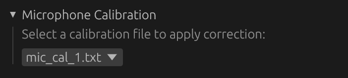
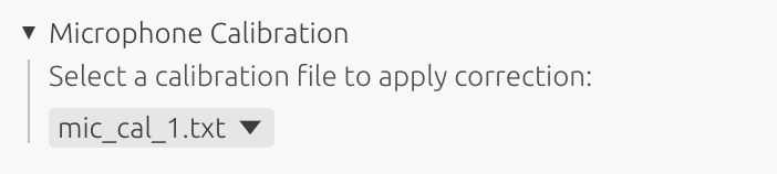
Microphone Calibration
Apply frequency response and sensitivity calibration corrections for your measurement microphone.
Overview
Each driver or room measurement can be assigned a microphone calibration that compensates for:
- Frequency response deviation from ideal flat response
- Sensitivity factor (dB conversion from microphone output to SPL)
Calibration management:
- Calibration files are managed in Settings → Mic Calibration (see Settings → Mic Calibration)
- Default calibration can be set for new drivers
- Each driver/measurement can use a different calibration or none at all
Calibration Dropdown
Location: Below the Driver/Measurement Name field
Options:
- None: No calibration applied (use for reference microphones or pre-calibrated measurements)
- [Calibration file names]: All imported calibration files from Settings → Mic Calibration
Behavior:
- Selection is saved with the project file
- Calibration data is stored in application settings, not in project files
- Changing the selection immediately recomputes the driver’s windowed IR and all filter responses
How Calibration is Applied
Processing pipeline:
- Measurement is imported and windowed (see Time Windowing)
- Microphone calibration correction applied (if selected)
- Minimum-phase FIR filter created from frequency response data
- Sensitivity factor (dB) applied as gain adjustment
- Frequencies below 5 Hz filtered out before processing
- Corrected IR used for all subsequent filtering (crossovers, correction filters, etc.)
Phase behavior:
- Correction uses minimum-phase reconstruction, affecting both magnitude and phase
- This is physically accurate for measurement microphones, which exhibit mainly minimum-phase behavior
Real-time updates:
- Calibration is recomputed whenever you change the windowing parameters
- Filter responses update automatically when you change calibration selection
When to Use Calibrations
Apply calibration when:
- Using consumer or measurement microphones with non-flat response
- You have calibration data from the manufacturer or third-party calibration service
- Measurements were taken with the same microphone used for the calibration file
Use “None” when:
- Measurements were taken with an already-flat reference microphone
- Importing measurements already compensated externally
Per-Driver vs. Default Calibration
Per-driver assignment (this window):
- Overrides any default set in Settings
- Useful when combining measurements from different microphones in one project
- Saved with the project file
Default calibration (Settings → Mic Calibration):
- Automatically applied to newly created drivers/measurements
- Does not affect existing drivers
- See Settings → Mic Calibration for configuration
Time Windowing
Isolate the direct sound from an impulse response and exclude reflections or noise.
Note: Time windowing is not available in Room Calibration mode. This is intentional: Room Calibration mode is designed to capture the full speaker-plus-room response, including reflections and room decay. Applying a time window would produce an anechoic-like impulse response — corrections derived from it would be wrong for the actual listening environment — what you hear is the direct sound from the speakers combined with all the reflections that follow, and the correction filters must account for that full response.

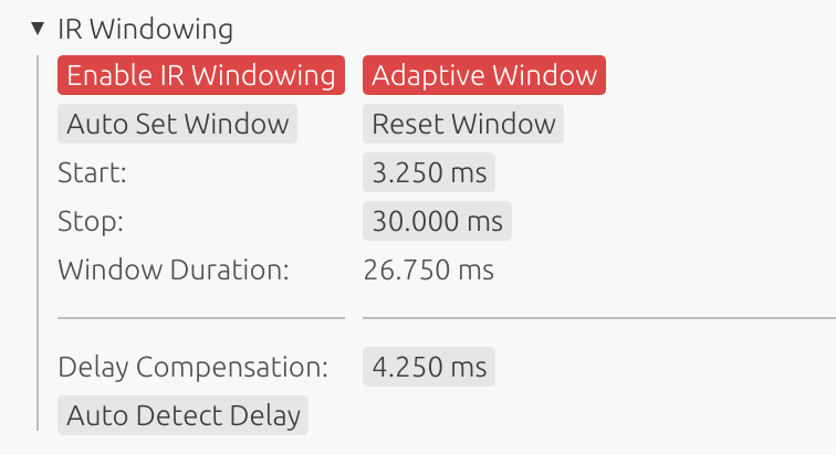
Parameters
Start Time
Beginning of the time window in milliseconds.
- Purpose: Remove pre-ringing or early noise
- Typical: 0.0 to 5.0 ms before main peak
- Effect: Sets the beginning of the extracted portion
Stop Time
End of the time window in milliseconds.
- Purpose: Exclude late reflections or room decay
- Typical: 5.0 to 100.0 ms after main peak
- Effect: Sets the end of the extracted portion
Duration Display
Wndow duration (Stop Time - Start Time).
Auto Set Window
Click “Auto Set Window” to automatically detect and configure optimal window boundaries.
How It Works:
The algorithm analyzes the on-axis measurement (0°, 0°) and automatically sets the start and stop times:
- Detect main peak: Locates the largest absolute amplitude in the impulse response
- Compute Hilbert envelope: Calculates the amplitude envelope for robust reflection detection
- Adaptive threshold: Adjusts detection sensitivity based on signal-to-noise ratio (3-8% of peak)
- Set start time: Places window start 3 ms before the main peak (clamped to 0.0 minimum)
- This margin accounts for off-axis measurements where the sound path may be shorter (gives a margin of ~1m)
- Prevents truncation of the direct sound in off-axis measurements
- Search for reflections: Scans the envelope for the first significant reflection/echo after the main peak:
- Must occur at least 3 ms after the main peak
- Must exceed the adaptive threshold
- Must be a local maximum in the envelope
- Set stop time: Places window stop 0.5 ms before the first detected reflection
If no significant reflection is detected, the stop time is set to the end of the search window or IR length.
Detection Method:
The algorithm uses Hilbert envelope analysis to detect reflections. This provides more robust detection than simple amplitude analysis by following the overall energy contour of the signal, making it less sensitive to oscillations within the waveform.
Window Margins:
- Start margin (3 ms): Ensures off-axis measurements are not truncated when rotating large loudspeakers. At the speed of sound (~343 m/s), 3 ms corresponds to approximately 1 meter of path length difference. During rotation, drivers may move closer to or further from the microphone—this margin provides sufficient safety for rotations of large cabinet.
- Stop margin (0.5 ms): Small margin before the detected reflection to avoid including the beginning of the echo.
Best Use Cases:
- ✅ Quasi-anechoic measurements: Ideal for measurements with clear, isolated reflections (e.g., outdoor, treated rooms, gated measurements)
- ✅ Controlled environments: Works well when the direct sound is clearly separated from reflections
- ✅ Multi-angle measurements: The 3ms start margin prevents truncation of off-axis measurements
- ✅ Time-saving: Quick initial window setup that can be manually refined if needed
Limitations:
- ❌ Reverberant environments: Not suitable for highly reflective rooms where reflections arrive continuously
- ❌ Dense reflection patterns: May not detect the first reflection correctly if multiple reflections arrive in quick succession
- ❌ Room measurements: For full-room measurements including reflections, manual windowing is more appropriate
Recommendation:
Use “Auto Set Window” as a starting point in quasi-anechoic conditions, then verify and adjust the window boundaries manually while observing the impulse response graph. In reverberant environments, set window parameters manually based on your measurement conditions.
Windowing Purpose
- Anechoic approximation: Simulate anechoic conditions from room measurements
- Reflection gating: Remove floor, ceiling, and wall reflections
- Crossover and correction design: Essential for accurate filter design using measured data
- Clean response: Isolate direct driver response
Window Function
LinFIR uses a Tukey window (tapered cosine/raised cosine) for smooth fade-in and fade-out transitions. This prevents spectral artifacts and high-frequency ringing caused by abrupt signal truncation.
Windowing Convention:
The fade-out starts at the stop parameter:
- Fade-in:
[start → start + taper] - Full signal:
[start + taper → stop] - Fade-out:
[stop → stop + taper]
Taper Duration: 0.5 ms for both simple and adaptive windowing
Preview
The impulse response graph shows the windowed result in real-time as you adjust start and stop times. The window boundaries are visually indicated.
Adaptive Window
Advanced frequency-dependent windowing that preserves low-frequency response while gating high-frequency reflections.
How It Works
When enabled, LinFIR uses a wavelet transform to apply different window lengths for different frequencies:
- Start parameter: Applied uniformly to all frequencies
- Stop parameter: Applied with frequency-dependent extensions
- Lower frequencies get longer decay times
- Higher frequencies use shorter windows
Examples of automatic extensions:
- 30 Hz: +33 ms beyond stop time
- 480 Hz: +2 ms beyond stop time
- 7.5 kHz: +0.1 ms beyond stop time
- 18 kHz: +0.06 ms beyond stop time
This reflects the physical reality that longer wavelengths make it difficult to temporally separate direct sound from reflections.
Benefits
- Preserves bass response: Low frequencies automatically get the time they need
- Avoids bass roll-off: Short windows don’t unnaturally cut off bass
- Frequency-aware gating: Removes high-frequency reflections while keeping bass intact
- No phase distortion: Maintains natural phase relationships
When to Use
Use Adaptive Window when:
- Gating reflections but need to preserve bass response
- Using short measurement windows where bass would be compromised
- Simple windowing causes unnatural bass attenuation
- You want frequency-dependent decay times matching physical acoustics
Don’t use Adaptive Window when:
- Working with anechoic or quasi-anechoic measurements with very clean direct sound (simple window is cleaner)
- You have sufficient window length for all frequencies uniformly
- You prefer uniform windowing for consistency
Enabling
Check the “Adaptive Window” checkbox in the IR Windowing section.
Delay Compensation
Shift the impulse response earlier in time without truncating data.
How It Works
- Non-destructive: IR data remains intact in memory
- Display offset: Delay applied as metadata for display and calculations
- Purpose: Bring acoustic peak closer to time zero to flatten the phase
Auto Detect Delay
Click “Auto Detect Delay” to automatically detect and apply optimal delay compensation across all drivers:
Behavior:
- Detects the peak position for each driver (based on on-axis measurements)
- Finds the minimum detected delay across all drivers
- Applies this minimum delay to all drivers simultaneously
Advantages:
- Preserves temporal alignment: All drivers maintain their relative timing relationships
- Removes common delay: Eliminates the shared propagation delay from all measurements
- Prevents errors: Ensures consistent delay compensation across all drivers automatically
Detection Method:
- Locates the position of the main peak in the impulse response
- Uses on-axis measurement (0°, 0°) as reference for each driver
- Aligns all driver peaks precisely at time zero
Manual Adjustment
Manually enter delay value in milliseconds to fine-tune compensation for individual drivers.
Sync Toggle (enabled by default):
When the Sync toggle is enabled, any manual delay adjustment automatically applies to all drivers in the project. This ensures consistent compensation across all drivers without needing to adjust each one individually.
- Enabled: Changes to the delay parameter propagate to all drivers automatically
- Disabled: Changes only affect the current driver, allowing independent delay values
- Activating Sync: If Sync is currently disabled and you enable it, an automatic delay detection is triggered to ensure all drivers have coherent delay values
When to use independently (Sync disabled):
- Only when drivers were measured with significantly different microphone positions
- Even then, prefer fixing microphone position and re-measuring rather than relying on delay compensation
Purpose and Limitations
What delay compensation is FOR:
- Removing the time of flight of sound from the measurement (optional, depends on personal preference)
- Correcting for different microphone positions between measurements
What delay compensation is NOT for:
- ❌ Time-aligning drivers during crossover design (this is handled separately by the Time Delay parameter)
- ❌ A tool for precise multi-driver coherence (proper crossover phase design is required instead)
Important: Microphone Position Corrections
Delay compensation can correct for microphone position differences, but this method has significant limitations:
⚠️ High-frequency measurement errors scale with wavelength:
- 10 cm microphone position difference → Errors above ~3400 Hz
- 5 cm microphone position difference → Errors above ~6900 Hz
- Ultra-short wavelengths (high frequencies) amplify measurement uncertainties
Best practice:
- ✅ Prefer re-measuring with fixed microphone placement rather than compensating for position differences
- ✅ Maintain consistent microphone position across all measurements when possible
- ✅ Delay compensation cannot replace careful measurement technique
Off-Axis Measurements:
- The selected delay compensation applies uniformly to all off-axis measurements (cannot vary by angle)
- This affects the relative timing between different measurement angles consistently
Measurement Notes
Section: Collapsible header (default closed) Purpose: Document measurement conditions and hardware setup
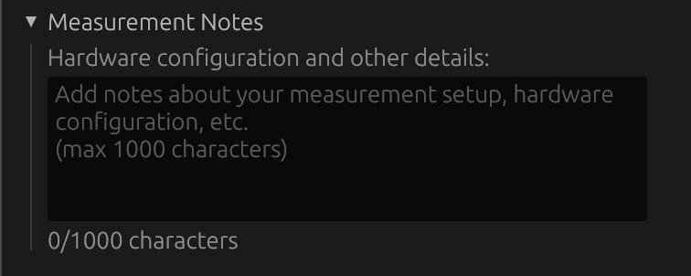

Overview
The Measurement Notes field provides a space to record important information about your measurement setup, hardware configuration, environmental conditions, and any other relevant details.
Features
- Multi-line text editor: Supports up to 1000 characters
- Auto-save: Notes are saved with the project
- Hint text: Helpful placeholder text suggests what information to include
- Character counter: Live display of character count (e.g., “127/1000 characters”)
What to Document
Hardware configuration:
- Microphone model and serial number
- Audio interface model and settings
- Amplifier configuration
- Cable connections and routing
Measurement conditions:
- Date and time of measurement
- Room conditions (temperature, humidity if relevant)
- Microphone position and distance
- Driver orientation and mounting
Reference information:
- Calibration file version used
- Sample rate and sweep settings
- Any unusual conditions or observations
- Version of measurements for tracking
Example Notes
Microphone: UMIK-1 (S/N: 123456) with cal file v2.3
Interface: Focusrite Scarlett 2i2 (48kHz, 512 buffer)
Distance: 1m on-axis, driver mounted in baffle
Room: Semi-anechoic (windows gated at 10ms)
Date: 2025-12-14
Notes: First measurement after driver break-in period
Best Practices
- Be specific: Include model numbers and serial numbers when relevant
- Date your measurements: Track when measurements were taken
- Note calibration: Record which calibration file was used
- Document changes: If re-measuring, note what changed
- Reference conditions: Record anything that might affect comparisons
Exporting Impulse Responses
Impulse responses can be exported individually or in batch using two methods:
Individual Export (Per-Measurement)
For each measurement (horizontal and vertical angles):
- Click the ⬇ (Export) button next to the measurement angle
- Export dialog appears with format options
- Choose export format (WAV or TXT) and options
- File is saved with automatic angle suffix
File naming format:
- Format:
DriverName_v{vertical}h{horizontal}.extension - Examples:
- On-axis (0°, 0°):
Driver 1_v0h0.wav - Horizontal +30°:
Driver 1_v0h30.wav - Vertical -15°:
Driver 1_v-15h0.wav - Horizontal -45°:
Driver 1_v0h-45.wav
- On-axis (0°, 0°):
Room Calibration mode (no angles):
- Format:
MeasurementName.extension - Example:
Measurement 1.wav
Batch Export (All Measurements)
Button: ⬇ Export All (above “Measurement angle” field)
Process:
- Click “⬇ Export All” button
- Select output directory in folder picker
- All measurements exported simultaneously as WAV files
- Files use consistent
v{vertical}h{horizontal}naming
Format (batch export):
- All files exported as WAV (32-bit float, mono)
- Sample rate matches project sample rate
- “Include distortion” option applies to all files
- No format selection (always WAV for batch)
Benefits:
- Fast export of complete measurement sets
- Consistent naming for re-import compatibility
- Files can be re-imported via batch import with automatic angle detection
- Compatible with external tools
Use cases:
- Archiving complete measurement sets
- Sharing measurements with collaborators
- External processing (FIR Designer, Matlab, REW)
- Backing up measurements before making changes
Export Format Options
When you click the export button, a dialog presents two format options:
WAV Format
File format:
- Channels: Mono
- Bit depth: 32-bit PCM float
- Sample rate: Project sample rate
Include Distortion Metadata option:
When checked:
- Exports full deconvolved IR plus custom ‘dist’ metadata chunk
- File name automatically gets
_dist.wavsuffix - Enables THD computation when re-imported into LinFIR
- Contains sweep parameters: start frequency, end frequency, duration
When unchecked:
- Exports only the active (cropped/windowed) working IR
- Standard WAV file without metadata
- Cannot be used for THD computation upon re-import
TXT Format
File format:
- One sample per line in scientific notation (e.g.,
1.234567e-03) - Metadata stored as comment lines starting with
#:# fs=<value>- Sample rate in Hz# IR data:- Marks the start of sample data
- Compatible with external tools (e.g., Matlab, Python)
- Can be re-imported into LinFIR
Include Distortion option:
TXT export does NOT support distortion export:
- The “Export as TXT” button is disabled when “Include distortion” is checked
- TXT format can only export the cropped IR (main impulse only)
- For distortion data export, use WAV format which supports embedded metadata
THD Availability
Total Harmonic Distortion (THD) graphs are only available when:
- IR was captured directly via LinFIR’s built-in sweep, or
- IR was imported from WAV with ‘dist’ metadata chunk (exported with “Include dist.” option in LinFIR)
Plain WAV files without ‘dist’ chunk or TXT files cannot produce THD curves.
Best Practices
For Captures
- Use proper gain staging to avoid clipping
- Monitor levels during sweep - aim for -6 dB to -12 dB peak
- Save captures with “Include dist.” for future THD analysis
For Windowing
- Use anechoic or quasi-anechoic measurements when possible
- Apply windowing before designing correction filters
- Check impulse response graphs to verify proper window placement
- Use Adaptive Window cautiously - verify bass response is realistic
For File Management
- Use descriptive IR names for organization
- Export with distortion metadata if you need THD analysis later
- Keep original unprocessed captures as backups
- Document measurement conditions (position, distance, etc.)
Quick Reference
| Action | Result |
|---|---|
| Import WAV | Load IR from WAV file (with or without ‘dist’ metadata) |
| Import FRD | Convert frequency response data to impulse response |
| Capture Sweep | Built-in measurement with automatic THD support |
| Time Windowing | Extract portion of IR, exclude reflections |
| Adaptive Window | Frequency-dependent windowing for bass preservation |
| Delay Compensation | Shift IR in time (non-destructive) |
| Export WAV | Save IR to WAV (with optional distortion metadata) |
| Export TXT | Export coefficients to text file |