
Kaiser Window
On this page
Every FIR filter of LinFIR is cut to a length, its number of taps, and each Kaiser β field sets how the filter is faded out towards its ends instead of being cut off abruptly. This page explains what that changes, and why a driver has several of these fields. The settings themselves are described with their windows: Kaiser β of the crossovers, of the corrections, and the Final Window β.
The Kaiser Window
A window is a weight given to each tap of the filter: 1 keeps the tap as it is, 0 removes it. Cutting a filter to N taps without a window is a window too, a rectangular one: 1 inside, 0 outside. The Kaiser window goes from 1 in the middle to a small value at the ends, more or less quickly depending on β:
$$w(x) = \frac{I_0\left(\beta \sqrt{1 - x^2}\right)}{I_0(\beta)}, \qquad x \text{ from } -1 \text{ (first tap) to } 1 \text{ (last tap)}$$
where \( I_0 \) is a Bessel function. β 0 is the rectangular window: no fading at all. The higher β, the narrower the window.
At its ends, the Kaiser window still weighs \( 1 / I_0(\beta) \): 0.79 at β 1, 0.06 at β 4.5. Below β 8 or so, the filter would stop on a step, which leaks across the whole spectrum and shows as a kink in the impulse response of the combined filter. So each filter LinFIR designs (crossovers and corrections) ends on a short fade as well, over the last 5% of each side, that brings its coefficients and their slope to 0; at β 0, the window is flat but for this fade.
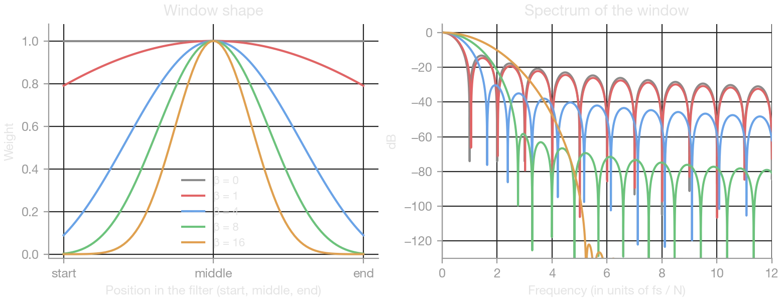
The right-hand plot is what the window does to a frequency response: windowing a filter smooths its response with this curve. Two things matter:
- The main lobe (the central bump): its width is how much the response is blurred. The narrowest is β 0.
- The side lobes (the ripples beside it): their level is how far the blurring leaks. This is what limits the depth of a stopband, and gives the ripple near a sharp transition.
| β | Main lobe (half width) | Highest side lobe |
|---|---|---|
| 0 | 1.0 × fs / N | −13 dB |
| 1 | 1.05 × fs / N | −15 dB |
| 4 | 1.6 × fs / N | −30 dB |
| 8 | 2.8 × fs / N | −58 dB |
| 16 | 5.2 × fs / N | −122 dB |
The main lobe's half width is \( \sqrt{1 + (\beta / \pi)^2} \) times fs / N: at 48 kHz and 4096 taps, fs / N is 11.7 Hz, so β 8 blurs the response over about ±33 Hz.
Time and Frequency: The Trade-Off
A filter of N taps lasts \( T = N / f_s \): 85 ms for 4096 taps at 48 kHz. Like any signal, it cannot be both short in time and sharp in frequency. This is the uncertainty principle of signal processing (Gabor): the spread of a signal in time, \( \Delta t \), and in frequency, \( \Delta f \), cannot both be small,
$$\Delta t \cdot \Delta f \geq \frac{1}{4\pi}$$
so a filter with a fixed length can only resolve frequency details down to about \( 1 / T \). The window shares out what the length allows: it shortens the filter's effective duration (the ends weigh less), which widens its frequency details, in exchange for a much lower leakage.
A brickwall low-pass shows it best: the ideal filter is a sinc that never ends, so cutting it to a length always costs something.
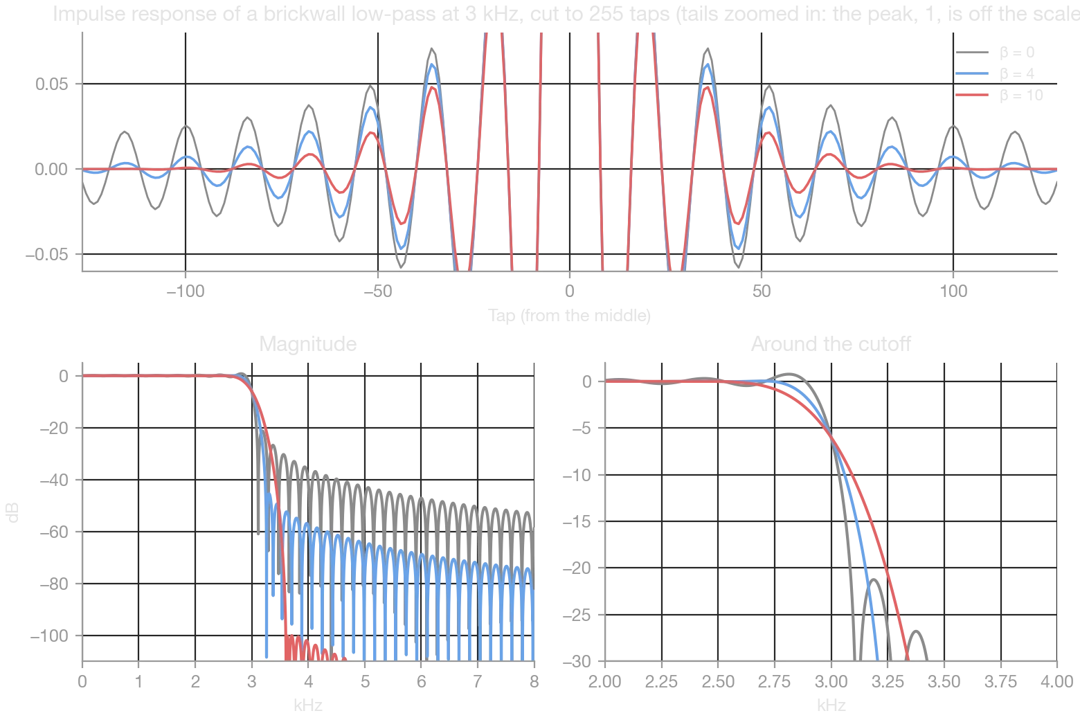
- β 0: the cut keeps the tails as they are, and stops them dead at the ends. The transition is the steepest, but the response overshoots by about 1 dB before the cutoff (Gibbs phenomenon) and the stopband stays between −20 and −55 dB.
- β 10: the tails fade out, the stopband goes below −100 dB, and the transition is about twice as wide.
- β 4: in between.
At a given length, β trades the steepness of the transitions and the sharpness of the corrections for the depth of the stopband. Only more taps give both. Kaiser's design formulas put figures on it: for a stopband attenuation of A dB,
$$\beta \approx 0.1102\,(A - 8.7) \quad (A > 50), \qquad \Delta f \approx \frac{(A - 7.95)\, f_s}{14.36\,(N - 1)}$$
where \( \Delta f \) is the width of the transition. For 60 dB (β ≈ 5.7): about 42 Hz at 48 kHz and 4096 taps, about 230 Hz at 93.75 kHz and 1500 taps (Hypex). This is why a low crossover, or a narrow correction in the bass, needs many taps.
Filters That Are Not Symmetric
A linear-phase filter is symmetric: its peak is in the middle, and a window centred on the middle fits it. A causal or mixed filter (Causality above 0) has its peak earlier, and a long tail after it. A window centred on the middle of such a filter would weigh its peak at less than 1, and leave its tail almost untouched.
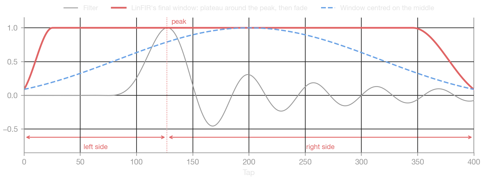
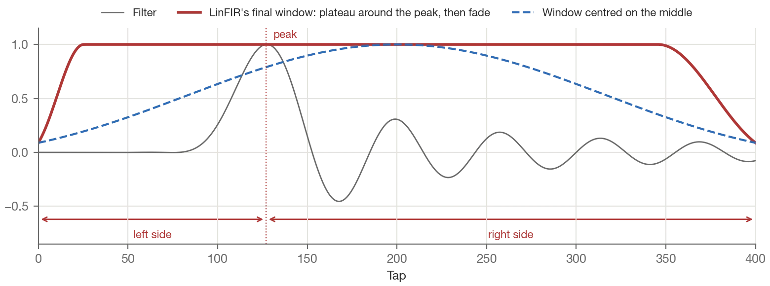
LinFIR's final window is centred on the filter's peak, and only fades out its ends: on each side of the peak, it leaves the first four fifths of the taps untouched, then fades the last fifth out with a half Kaiser window. A causal filter keeps its peak at 1, and each side fades out over the room it has.
Why Several Windows
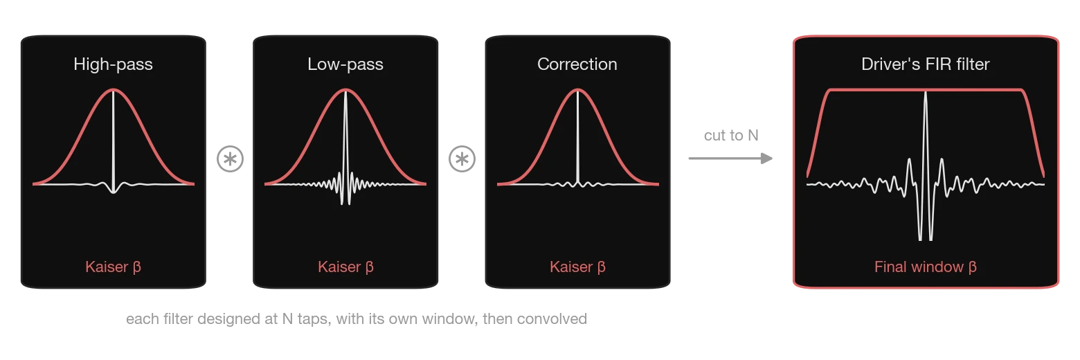
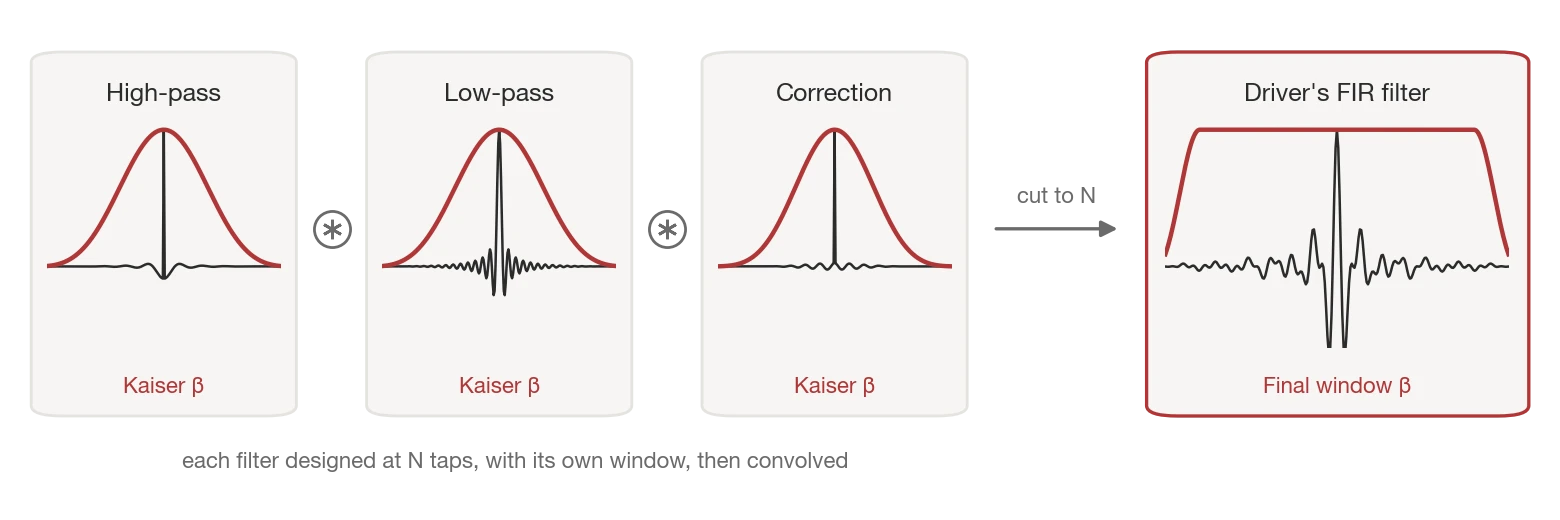
A driver's FIR filter is made of several filters: high-pass, low-pass, magnitude correction and phase correction. LinFIR designs each one at the filter length with its own window (its Kaiser β field), convolves them, cuts the result to the filter length, and applies the final window (the Final Window β field) to the result.
In Plain Words
Think of each filter as the recording of a note, and of its length as the time the recording lasts.
- A note that has died out before the end can be cut anywhere: nothing is lost, and its window hardly matters.
- A note still sounding at the end is cut in the middle, and the cut is heard as a click. That click is leakage: sound spread over frequencies where the filter should be silent.
- A window fades the note out before the end instead: no click, but the end of the note is lost, and the filter is less precise. That is the whole trade-off of β.
Convolving filters is like playing one recording through the others: a click in one of them goes through all of them. The final window fades out the end of the combined result: it softens the clicks that land there, but when the filters fill the whole length, as short filters do, the fade also cuts into the notes themselves.
How the Windows Combine
Convolving filters multiplies their responses, so each filter's leakage and each filter's loss of detail end up in the combined filter:
- A filter cut almost rectangular (low β) keeps all its detail. If its impulse response still oscillates at its ends, though, its leakage goes into the combination, and the final window only attenuates it as much as it fades the ends: a gentle final window lets most of it through.
- A final window fades out what lands at the ends of the combined filter. When the filters still sound there, it also cuts into them: the crossovers' transitions widen, and the response rises past the crossovers above the designed slope.
- A high β on every filter blurs each of them, and the blurs add up: narrow corrections and steep crossovers come out less precise than the length allows.
Recommendations
- Leave the final window at 0, the default: the combined filter is cut without a window, and the crossovers keep the slopes their own windows give them.
- Raise it only for a driver whose response leaks past its crossovers, typically a driver between two crossovers with short filters, and look at the result: if the response past the crossovers rises above the slope it had at 0, lower it again. Values from 2 to 4 are the ones that helped in our tests.
- The filters' own windows do the rest. A filter that still rings at its ends (a low crossover, a steep or brickwall one, a narrow correction in the bass) needs its own Kaiser β; the others can be permissive (a low β), since their impulse response dies out within the length and a window would only take detail away.
- The filter that leaks is also the one that needs the length most: a stronger window lowers its leakage at the cost of its own precision. When that precision matters (a narrow correction in the bass), more taps are the only way to have both.
The global correction has the same pair of settings: the Kaiser β of its magnitude and phase corrections, and its own final window β.