
Directivity Analysis License
On this page
- Overview
- Polar Measurements
- Off-Axis Curve Visualization
- Directivity Index (DI) Prediction
- Listening Window
- Predicted In-Room Response
- Early Reflections, Sound Power and Early Reflections DI
- Directivity Analysis Window
- Overlay Plot Tab
- Preserving Time-of-Flight
- Limitations and Best Practices
- Getting a License
- Related Documentation
- Summary
License Required: Directivity analysis features require a valid LinFIR license. All other LinFIR features remain free to use.
Directivity analysis tools characterize how your speaker system radiates sound in different directions. These tools predict off-axis behavior, visualize interference patterns between drivers, and help optimize crossover design for consistent directivity.
Overview
Directivity analysis provides:
- Off-axis frequency response visualization at any measured angle
- Directivity Index (DI) prediction across the frequency spectrum
- Directivity sonograms (2D frequency vs. angle heatmaps)
- Crossover optimization insights based on radiation patterns
Key Applications:
- Identify directivity errors, beaming and dispersion characteristics
- Optimize crossover design for consistent off-axis response
- Assess room interaction based on directivity patterns
- Visualize interference patterns between drivers
Polar Measurements
Measurement Requirements
To use directivity tools, you need impulse responses at multiple angles:
Horizontal Axis:
- Measurements with vertical angle = 0°, varying horizontal angle
- Example: -90°, -60°, -30°, 0°, +30°, +60°, +90°
- More angles provide better accuracy (5° or 10° increments recommended)
Vertical Axis:
- Measurements with horizontal angle = 0°, varying vertical angle
- Example: -60°, -40°, -20°, 0°, +20°, +40°, +60°
- Particularly important for speakers with vertical array configurations
On-axis Reference:
- The (0°, 0°) measurement is the on-axis reference
- Must be captured first before off-axis measurements
- Appears in both horizontal and vertical columns in the IR Management window
Calculation distance:
- Every directivity result - the off-axis curves, the Listening Window, the Predicted In-Room Response, Early Reflections, Sound Power, the DIs and the sonogram - is calculated at the project's calculation distance: the drivers' paths and angles as from a listener at that distance from the reference point
- 2 m in a new project, as ANSI/CTA-2034-A measures; a project from before 1.5.2 stays at its measurement distance
- Set once for the project in the IR window, polar mode, Enclosure section - see The calculation distance
⚠️ Critical: Time of Flight Must Be Preserved
DO NOT:
- Apply windowing that removes the acoustic delay
- Time-align measurements to the same start point
- Remove the relative delay between drivers
WHY:
- The relative delay between angles encodes interference patterns
- This delay represents the acoustic path length to the microphone
- Off-axis measurements have different path length ratios between drivers
- These delays create the directivity patterns we analyze
What happens if you remove time-of-flight:
- DI calculation assumes drivers are co-located (incorrect)
- Predicted interference patterns don't match reality
- Off-axis nulls and peaks won't appear
- Directivity sonograms show incorrect lobing patterns
⚠️ Critical: Use Proper Timing Reference
Configure a timing reference method in Audio Settings before capturing polar measurements:
Electric (loopback) - RECOMMENDED:
- Most reliable method
- Connect output to input with a cable
- Eliminates software scheduler variability
- See Reference Timing for setup
Acoustic (chirp):
- Uses another driver as timing reference microphone
- Good for setups where loopback is impractical
- Requires careful positioning
Avoid "None" timing mode:
- Relies on system audio scheduler (unreliable on Windows)
- Timing jitter corrupts phase relationships between drivers
- Can produce incorrect directivity analysis
💡 Tip: Stable timing is essential for accurate phase relationships between drivers. See Reference Timing for detailed setup instructions.
Automated Polar Measurements with a Rotation Table
For a fully automated polar measurement workflow, connect a motorized turntable (Pololu Tic or GRBL/Arduino) in Settings → Rotation Table. Once connected and a license is active:
- A ▶ Scan button appears in the IR Management window
- Configure the angle range and step (e.g. −90° to +90°, 10° step)
- Click ▶ Scan: the table rotates to each angle, settles, and captures automatically
- Already-measured angles are skipped
See Rotation Table for setup, hardware compatibility, and troubleshooting.
Measurement Tips
General Guidelines:
- Keep microphone-to-speaker distance constant for all angles
- Rotate the speaker (not the microphone) when possible
- Ideally the speaker turns about its front baffle; when the turntable axis is behind it (or off to the side), set the enclosure and its turntable placement in the IR Management window's polar mode so LinFIR rebuilds the off-axis responses at the right distance and angle - see The Enclosure and the Rotation Center
- Ensure consistent room conditions for all measurements
- Use high SNR settings to capture clean off-axis data
Distance Recommendations:
- Farfield measurements (>1 meter) work best
- Distance should be at least 2-3× the largest driver spacing
- Too close = nearfield effects, inaccurate directivity
- Too far = room reflections dominate
Microphone Positioning:
- Ensure microphone height matches speaker acoustic center
- Keep microphone axis perpendicular to speaker front baffle
- Avoid obstructions in the measurement path
Off-Axis Curve Visualization
View off-axis frequency responses directly in the main graph window.
Accessing Off-Axis Display
Location: Main graph toolbar (Drivers/Speakers display mode only)
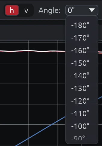
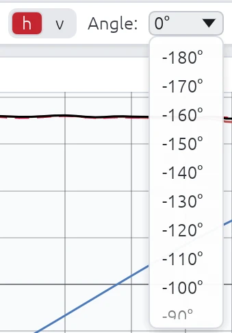
Axis Selection:
- Toggle between h (horizontal) and v (vertical) axis buttons
- Only available when viewing individual drivers or summed system
- Not available in Room Calibration modes
Angle Dropdown:
- Select from available measurement angles
- Only angles with actual measurement data are shown
- 0° always represents the on-axis reference
Interpreting Off-Axis Curves
Compare off-axis to on-axis:
- Smooth transitions across angles = good dispersion control
- Large deviations at certain angles = beaming or nulls
- Crossover region consistency = proper driver integration
What to look for:
- Beaming: Response drops off rapidly at off-axis angles (high-frequency issue)
- Comb filtering: Peaks and dips that vary with angle (driver interference)
- Crossover lobing: Nulls or peaks appearing at specific off-axis angles near crossover frequency
- Baffle diffraction: Ripples that change with angle at mid-to-high frequencies
Example Interpretation:
Good directivity:
- Off-axis curves smoothly roll off at high frequencies
- No sudden dips, peaks or steps through crossover region
- Consistent shape across ±30° angles
Poor directivity:
- Deep nulls appearing at ±20° near crossover frequency
- Off-axis step in frequency response near a crossover frequency, indicating directivity mismatch between drivers
- Dramatic level changes between neighboring angles
- Comb filtering visible at mid frequencies
Directivity Index (DI) Prediction
The Directivity Index (DI) quantifies how directional your speaker is across the frequency spectrum.
What is DI?
Definition:
LinFIR's DI is the Sound Power Directivity Index (SPDI) of the ANSI/CTA-2034-A standard: the Listening Window level minus the Sound Power level.
\[ \text{DI} = 20 \log_{10} \frac{\text{LW}}{\text{SP}} = \text{LW (dB)} - \text{SP (dB)} \]
The classic acoustic definition, \(10 \log_{10} Q\) with the directivity factor \(Q\), compares the on-axis intensity with the average over the whole sphere. The standard references the Listening Window instead - the sound most listeners actually get - so a narrow on-axis peak or dip doesn't show up as a change of directivity. The two differ mostly in the treble, where the drivers narrow and the Listening Window falls below the on-axis response.
\(\text{LW}\) and \(\text{SP}\) are computed from the acoustic sum of all the active drivers at each measured angle - each with its filters, gain, delay and polarity, phase included - the same summed response the Predicted In-Room curve uses. Interference between drivers is therefore part of the DI.
Interpretation:
- 0 dB = omnidirectional (radiates equally in all directions)
- Higher values = more directional (sound focused forward)
Typical DI Values
0-3 dB: Wide dispersion
- Subwoofers
- Large woofers at low frequencies
- Most speakers below 200 Hz
3-6 dB: Moderate directivity
- Most drivers at mid frequencies
- Typical 2-way speakers at 1-4 kHz
6-12 dB: Controlled directivity
- Waveguides and horns
- Well-designed constant directivity systems
- Ideal for controlled room interaction
12+ dB: Very directional
- Narrow dispersion (potential beaming issues)
- Extreme horns
- May sound disconnected from room in typical listening spaces
How DI Reflects Filtering
The DI curve shows:
- Combined effect of driver placement and crossover filtering
- Interference between drivers creates peaks/dips in the DI
- Crossover slopes affect how quickly directivity changes
- Time-of-flight differences encode driver spacing in the DI pattern
Example DI Behaviors:
Smooth DI transition:
- Gradual increase from 3 dB at 500 Hz to 6 dB at 4 kHz
- Indicates good driver integration through crossover
DI spike at crossover:
- Peak to 8-10 dB at 2.5 kHz, then drops to 6 dB at 3 kHz
- Indicates a summing peak (lobing) in the listening window at crossover frequency
- Off-axis response likely has nulls
DI dip at crossover:
- Dip to 0 dB at crossover frequency
- Indicates a null (destructive interference) in the listening window
- The cancelled energy goes to other directions, where it may sound better
Using DI for Design
Target smooth DI transition:
- Avoid sudden changes (>3 dB) in DI through crossover region
- Gradual transitions indicate good driver integration
Avoid sudden DI changes:
- Peaks = forward lobing (hot spot)
- Dips = forward null (cancellation)
- Both indicate poor crossover alignment
Consider desired room interaction:
- Wider DI (3-6 dB) = more room sound (spacious, diffuse)
- Narrower DI (6-12 dB) = less room sound (direct, focused)
- Match DI to listening environment and preference
Match DI to listening environment:
- Near-field (desktop, mixing): Moderate DI acceptable (3-8 dB)
- Far-field (living room, theater): Wider DI preferred (3-6 dB) to engage room
- Treated rooms: Higher DI acceptable (6-10 dB) due to controlled reflections
Display Requirements
The DI curve is shown in the Frequency Responses (Drivers) graph when:
- A valid LinFIR license is active
- At least one enabled driver has off-axis measurements
- The Directivity Index toggle is enabled, in the Graphs dropdown's Overlays section (per-project; Settings → Graphs → Default Overlays sets what a new project starts with)
- The Drivers display mode is selected in the graph toolbar
Listening Window
The Listening Window curve represents the average frequency response over the angular range that matters most for typical listening positions — the region a listener's ears are likely to be within.
What is the Listening Window?
The Listening Window is defined as the power average of all measured frequency responses within ±30° horizontal and ±10° vertical (inclusive) - the root of the mean of the squared magnitudes, as CTA-2034-A §5.2 prescribes for all its averages. For the standard's 10° orbits these are its nine directions: 0°, ±10° vertical and ±10°, ±20°, ±30° horizontal. It captures the sound power arriving at listeners seated slightly off-axis, which is more representative of real-world listening conditions than the strict on-axis response alone.
Display Requirements
The Listening Window curve is shown in the Frequency Responses (Drivers) graph when:
- A valid LinFIR license is active
- At least 2 polar measurements fall within the ±30° horizontal / ±10° vertical window
- The Drivers display mode is selected in the graph toolbar
Visual Appearance
| Property | Value |
|---|---|
| Color | Royal blue (fixed) |
| Line style | Dashed |
| Label | LW |
The dedicated color and dashed style let the Listening Window be picked out at a glance among the Sum, DI, Predicted In-Room Response and per-driver curves on the same plot. The Sum curve is always drawn on top, so it's never hidden underneath. Hovering the curve shows its full name, "Listening Window", in the tooltip - the legend stays compact ("LW").
Interpreting the Listening Window
LW ≈ Sum (on-axis):
- The speaker's balance changes little within the listening window
- Indicates excellent controlled directivity in the ±30°H / ±10°V region
- High confidence that off-axis listeners experience a similar tonal balance
LW rolls off above Sum at high frequencies:
- Normal and expected behaviour (drivers beam at high frequencies)
- The high-frequency roll-off shape indicates how quickly the speaker narrows
- A gentle, smooth roll-off indicates controlled directivity
LW has dips or irregularities not present on-axis:
- Lobing, comb filtering or directivity discontinuities within the listening window
- May indicate a crossover alignment issue affecting near-axis radiation
- A sudden dip at a specific frequency often points to interference between drivers
Comparing LW with DI:
- As DI rises, the LW typically diverges from the on-axis Sum (more directional → more off-axis loss)
- A flat DI with a flat LW indicates a well-controlled constant-directivity design
Predicted In-Room Response
The Predicted In-Room Response (PIR) curve estimates what a typical domestic room's in-room measured response would look like, computed entirely from the anechoic (or gated) polar measurements already used for DI and the Listening Window — no actual in-room measurement is required.
This curve, together with the Listening Window and DI above, follows the ANSI/CTA-2034-A standard (formerly CEA-2034, the "spinorama" measurement suite) — the same standard used by AES/Harman loudspeaker research and by third-party spinorama tools, so PIR curves produced here are directly comparable to published third-party spinoramas built to the same standard.
What is PIR?
CTA-2034-A (§13) defines PIR as a fixed-weight combination of three curves, each itself a power average over a standard set of measurement angles. The weights apply to squared pressures, not to levels or magnitudes:
\[ \text{PIR} = \sqrt{0.12 \cdot \text{LW}^2 + 0.44 \cdot \text{ER}^2 + 0.44 \cdot \text{SP}^2} \]
LW — Listening Window: the same ±30°H / ±10°V power average described above.
ER — Early Reflections: the power average of the five standard first-reflection paths a listener's room would generate — Floor Bounce, Ceiling Bounce, Front Wall, Side Wall and Rear Wall — each itself the power average of the standard angles for that path:
Sub-curve Angles Floor Bounce Vertical −20°, −30°, −40° Ceiling Bounce Vertical 40°, 50°, 60° Front Wall Horizontal 0°, ±10°, ±20°, ±30° Side Wall Horizontal ±40°, ±50°, ±60°, ±70°, ±80° Rear Wall Horizontal ±90°, 180° A sub-curve with no matching measurement is left out of the average entirely (not treated as silence) — a driver measured out to only ±60° still produces a partial Early Reflections curve (Floor/Ceiling/Front/Side), just without the Rear Wall contribution. At least 3 of the 5 sub-curves must have data for Early Reflections — and therefore PIR — to be computed at all. A direction measured twice (−180° and 180°) counts once.
SP — Sound Power: the weighted power average of the measurements on the horizontal and vertical orbits (the standard's 70 directions at 10° steps), each weighted by the part of the sphere it stands for - see Sound Power below.
All three are computed at every frequency of the measurements, so the PIR curve stays dense and evenly spaced — required both for a smooth plot and for using PIR as a correction/Auto-EQ reference.
The 0.12 / 0.44 / 0.44 weighting reflects, on average, how much of a typical listening room's measured response is dominated by direct sound versus early reflections versus the reverberant field — the same figures published in the CTA-2034-A standard and the Olive/Harman AES research behind it.
Display Requirements
The Predicted In-Room Response curve is shown in the Frequency Responses (Drivers) graph when:
- A valid LinFIR license is active
- Early Reflections data is available (at least 3 of the 5 sub-curves above have a matching measurement)
- The Predicted In-Room Response toggle is enabled, in the Graphs dropdown's Overlays section (per-project; Settings → Graphs → Default Overlays sets what a new project starts with)
- The Drivers display mode is selected in the graph toolbar
Visual Appearance
| Property | Value |
|---|---|
| Color | Cherry red (fixed) |
| Line style | Dashed |
| Label | PIR |
PIR reflects the currently active global IIR/FIR correction filters, unlike DI, whose ratio a uniformly-applied filter cancels out of - so PIR moves when you adjust global filters, the same way the Sum curve does. Hovering the curve shows its full name, "Predicted In-Room Response", in the tooltip - the legend stays compact ("PIR").
PIR can also be selected as the Reference for the global magnitude correction filter and global Auto EQ, alongside On-axis and Listening Window - see System Processing.
Interpreting PIR
PIR close to LW:
- The speaker's off-axis energy tracks its near-axis balance closely
- Indicates well-controlled directivity across a wide angular range, not just the narrow listening window
PIR rolls off faster than LW at high frequencies:
- Expected for most speakers: as directivity narrows with frequency, less high-frequency energy reaches the room as a whole
- A smooth, gradual roll-off (rather than a sharp step) generally reads as more natural in a real room
PIR dips or bumps not present in LW or DI individually:
- Usually an Early Reflections effect specific to the floor/ceiling/side/rear angle sets — check the per-sub-curve angles if measurements are sparse there
- A partial Early Reflections curve (missing the Rear Wall sub-curve, for instance) can shift PIR slightly versus a full-coverage measurement; wider polar coverage narrows this
Early Reflections, Sound Power and Early Reflections DI
Early Reflections and Sound Power are the two sub-curves PIR combines above — each can also be shown on its own, alongside a third curve, Early Reflections DI, which isn't part of the PIR formula but completes the standard spinorama's set of directivity-index curves. Unlike Sum, Listening Window, PIR and DI, all three are hidden by default — turn them on individually from the Graphs dropdown's Overlays section if you want them.
Early Reflections (ER)
The power average of the five standard first-reflection sub-curves described under Predicted In-Room Response above — Floor Bounce, Ceiling Bounce, Front Wall, Side Wall, Rear Wall. Same availability rule as PIR: at least 3 of the 5 sub-curves need a matching measurement.
Sound Power (SP)
The sound power the loudspeaker radiates, expressed as the level of the equivalent average pressure. CTA-2034-A (§5.2 and Appendix C) computes it from the horizontal and vertical orbits: the squared magnitude of each measurement is weighted by the area of the spherical quadrangle around its direction, and the weighted mean is converted back to a level:
\[ \text{SP} = \sqrt{\frac{\sum_i w_i , |H_i|^2}{\sum_i w_i}} \]
- Weights: the standard's Appendix C tables - Table 7 for 10° steps (from 0.0006 on and behind the axis to 0.0196 at ±90°), Table 8 for 5° steps. For any other step (15°, 30°...) LinFIR uses the construction behind Table 7: the area between the spherical squares of half-width
angle ± step/2around the axis, shared by the four directions at that angle. The step is the largest one that fits every measured angle. - One orbit only - a turntable measurement without turning the loudspeaker on its side: the other orbit is taken as identical, so a horizontal-only measurement gives the Sound Power of a loudspeaker with the same directivity vertically. Measure the vertical orbit too when the drivers are stacked: their vertical interference changes the Sound Power.
- Missing angles are left out, and the weights of the measured ones normalized. Measurements off the two orbits (a full-sphere grid) aren't part of the standard's Sound Power and are not used.
DI is the Listening Window minus this curve, in dB.
Early Reflections DI (ERDI)
Listening Window (dB) − Early Reflections (dB), as CTA-2034-A §5.2 defines it — the counterpart of DI (the Sound Power DI, Listening Window − Sound Power) for the Early Reflections curve. Together they are the two directivity indices of the standard spinorama plot.
Display Requirements
Each curve is shown in the Frequency Responses (Drivers) graph when:
- A valid LinFIR license is active
- The underlying data is available (Early Reflections and Early Reflections DI need at least 3 of the 5 sub-curves above; Sound Power needs at least one measurement on the horizontal or vertical orbit)
- Its own toggle is enabled, in the Graphs dropdown's Overlays section (per-project; Settings → Graphs → Default Overlays sets what a new project starts with — all three default to off)
- The Drivers display mode is selected in the graph toolbar
Visual Appearance
| Curve | Color | Line style | Label |
|---|---|---|---|
| Early Reflections | Purple (fixed) | Dashed | ER |
| Sound Power | Teal (fixed) | Dashed | SP |
| Early Reflections DI | Dark orange (fixed) | Solid | ERDI |
Early Reflections and Sound Power are linear-magnitude curves, plotted the same way as Listening Window/PIR. Early Reflections DI, like DI, is already a dB ratio — it's offset upward into the same band of the plot as DI so both stay readable together, and the hover tooltip subtracts the offset back out to show the real value. Hovering any of the three shows its full name in the tooltip — the legend stays compact ("ER"/"SP"/"ERDI").
Directivity Analysis Window
The Directivity Analysis window displays two complementary visualizations of how sound radiates across frequency and angle. It is organized into two tabs:
- Sonogram — colour-mapped 2D heatmap (frequency × angle)
- Overlay Plot — all off-axis curves superimposed on a single frequency-response graph
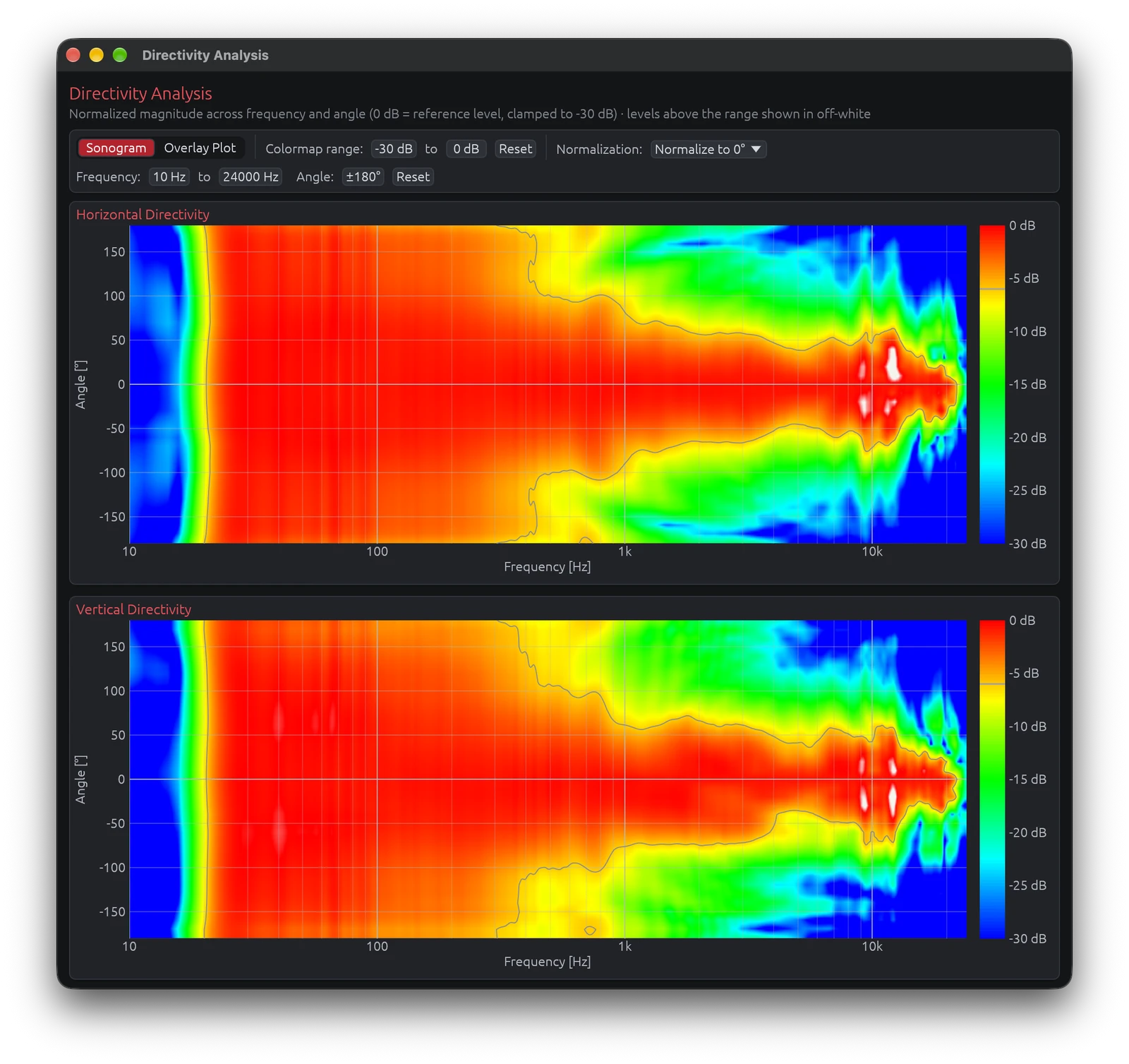
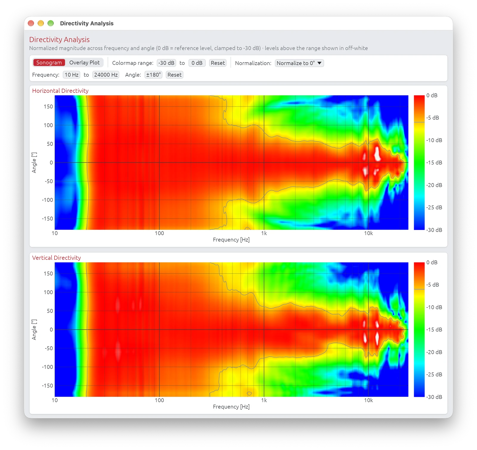
Accessing the Window
Menu: View → Directivity Analysis Requires: Valid LinFIR license and polar measurements loaded
Sonogram Tab — Layout
Two separate sonogram plots:
- Horizontal directivity: Vertical angle = 0°, varying horizontal angle
- Vertical directivity: Horizontal angle = 0°, varying vertical angle
Axes:
- X-axis: Frequency (Hz, logarithmic scale)
- Y-axis: Measurement angle (degrees)
- Color: Normalized magnitude in dB (0 dB = reference level, depending on normalization mode)
-6 dB Directivity Curves:
Thin grey overlay lines trace the -6 dB point on both sides of boresite (positive and negative angles) across frequency. These curves mark the angular width where the response stays within 6 dB of the on-axis maximum — a standard measure of directivity or "beamwidth."
- Wider grey-line separation at a given frequency → wider dispersion (omnidirectional behaviour)
- Narrower separation → more focused, beamed radiation
These curves make it easy to spot frequency ranges where the speaker narrows its dispersion (beaming) or where directivity becomes asymmetric between left/right and up/down.
Color Scale
Hot colors (red/yellow): Higher magnitude (0 dB and above)
- On-axis or near-axis energy
- Focused radiation
- With normalization modes, values above 0 dB indicate angles/frequencies stronger than the reference
Warm colors (orange): Moderate attenuation (-6 to -12 dB)
- Moderate off-axis output
- Typical dispersion
Cool colors (blue/purple): Significant attenuation (-12 to -30 dB and below)
- Heavily attenuated off-axis
- Beaming or nulls
Range clamped to -30 dB by default for clarity (adjustable in settings). The color scale always stops at 0 dB by default — increase the max dB threshold to extend it.
By default, values above the max threshold are drawn in off-white rather than saturating to the same red as the loudest in-range energy, so it stays obvious where a normalization mode pushes the response over the reference level. The shift is progressive — over-range pixels fade from red into off-white across about 1 dB above the threshold rather than switching colour on a hard edge, so there is no abrupt line in the image. Turn this off in Settings → Graph Settings → Highlight sonogram clipping to have over-range values saturate to red instead.
Colormap Range Controls
The Colormap range row in the sonogram toolbar lets you saturate the colour scale to reveal low-amplitude detail without reloading any measurement data.
| Control | Description |
|---|---|
| Min dB (drag-value) | Lower saturation threshold — anything at or below this value is rendered in cold blue |
| Max dB (drag-value) | Upper saturation threshold — anything at or above this value is rendered in hot red (or off-white when Highlight sonogram clipping is on, see Color Scale) |
| Reset button | Restores min to the configured magnitude lower bound and max to 0 dB |
How to use it:
- Widen the range (e.g. −60 dB to 0 dB) to get a broad overview of the full dynamic range
- Narrow the range (e.g. −15 dB to −5 dB) to zoom in on mid-level detail and expose subtle lobing or diffraction artefacts that would otherwise blend into a unique color
- Changing either value triggers an immediate image regeneration; the previous image remains visible while the new one is computed
The colorbar on the right of each sonogram always reflects the current min/max values and its grid step adapts automatically to the selected range.
Normalization Mode
The Normalization dropdown on the right side of the toolbar controls how sonogram magnitudes are normalised before applying the colour map. Four modes are available. The mode the sonogram opens with is set by Settings → Graph Settings → Sonogram normalization; the toolbar dropdown then overrides it for the current session.
| Mode | Description |
|---|---|
| Global max. | The entire sonogram is normalised to the single strongest magnitude found anywhere in the data, capped at 20 kHz to avoid tweeter resonance peak. Every pixel is expressed relative to that one global maximum — the brightest point in the whole image is always ≥0 dB. |
| Normalize to 0° | A single reference value is computed from the 0° (on-axis) row: the maximum magnitude found on-axis across all frequencies (capped at 20 kHz to avoid tweeter resonance peak). Every pixel is then expressed relative to that one value. With this mode, angles stronger than the on-axis reference will show positive dB values (displayed in red, saturated at the top of the color scale). |
| Normalize to 0° (per freq) | For each frequency independently, the response is normalised to the magnitude at 0° for that same frequency. Each frequency column therefore has its own 0 dB reference, which makes relative directivity patterns within each band immediately visible. On-axis at every frequency will appear at 0 dB, and off-axis deviations are shown relative to the on-axis response at that exact frequency. Positive dB values can appear where off-axis response exceeds on-axis at a given frequency. |
| Normalize to ±10° avg (per freq) | For each frequency independently, the response is normalised to the average magnitude between −10° and +10° at that frequency. Like "Normalize to 0° (per freq)" each column has its own 0 dB reference, but the reference is an average over a small angular window rather than a single on-axis point. This is more robust when the on-axis response has narrow peaks or dips caused by interference or diffraction. |
When to use which:
- Global max. — Quick overview of the full dataset
- Normalize to 0° — Comparing on-axis vs. off-axis directivity with a single reference. Useful for checking dispersion consistency
- Normalize to 0° (per freq) — Detailed analysis of angular directivity patterns per frequency band; removes the dependency on the driver's frequency response to compare with FEM/BEM simulations
- Normalize to ±10° avg (per freq) — Same as "Normalize to 0° (per freq)" but more robust against narrow on-axis anomalies. Prefer this when the 0° measurement has sharp peaks or nulls from interference patterns (e.g. driver spacing comb filtering) that would distort the per-frequency reference
Note on the 20 kHz cap: The reference maximum is always computed from frequencies at or below 20 kHz. This avoids tweeter resonance peaks in the ultrasonic range from skewing the normalization reference, which would otherwise compress the visible dynamic range in the audible band.
Interpreting Sonograms
Horizontal bands:
- Similar spectral balance across angles
- A band remaining coherent from about −60° to +60° indicates a well-designed driver with controlled directivity and no excessive beaming
Angular width and color spread:
- Warm colors extending from −90° to +90° in the bass / low-midrange are normal (low frequencies are inherently near-omnidirectional)
- Progressive narrowing at high frequencies is expected, but confinement to < −45° to +45° suggests excessive beaming
Symmetry around 0°:
- Geometrical and acoustical symmetry
- Proper driver placement and reliable measurements
Asymmetric patterns:
- Potential baffle diffraction
- Room reflections contaminating measurements
- Driver offset or asymmetric waveguides (intentional in most 3 way monitor designs)
Interference patterns (diagonal/complex):
- Driver interaction visible
- Crossover region summing effects
- Time-of-flight encoding driver spacing
What to Look For
Good Patterns:
Smooth color transitions:
- Gradual change from hot (on-axis) to cool (off-axis)
- Indicates controlled directivity
Symmetric patterns:
- Equal radiation to left/right (horizontal) or up/down (vertical)
- Indicates Symmetric design
Horizontal bands in crossover region:
- Consistent radiation pattern through crossover
- Good driver integration
Bad Patterns:
Narrow bright vertical regions:
- Beaming (concentrated energy on-axis)
- Excessive directivity at that frequency
- Often caused by large drivers at high frequencies
Dark spots off-axis / Diagonal stripes:
- Nulls or cancellations between drivers
- Indicates poor crossover alignment or lobing
- May be acceptable if smooth and symmetric
- Often caused by driver spacing and time-of-flight
- Crossover regions with insufficient acoustic slope, producing off-axis lobing
Crossover Design Insights
Compare on-axis and off-axis patterns:
- Check for consistent summing across all angles
- Look for lobing (bright spots appearing at off-axis angles)
Verify driver summing:
- Crossover frequency should show smooth transition in sonogram
- Moderate nulls or peaks appearing at specific angles
Adjust crossover if needed:
- Lobing visible: Try different crossover slopes or frequency
- Nulls visible: Check driver polarity and time alignment
Example Adjustments:
Problem: Bright and wide lobe at +30° near crossover frequency Solution: Lower crossover frequency or increase slope to reduce overlap
Problem: Null at 0° (on-axis) at crossover frequency Solution: Check driver polarity, adjust time delay, or change crossover type
Problem: Vertical bright bands alternating with dark bands Solution: Driver spacing issue (comb filtering) - may require physical redesign
Overlay Plot Tab
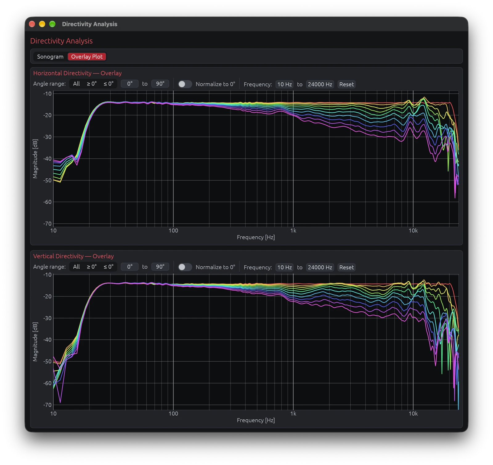
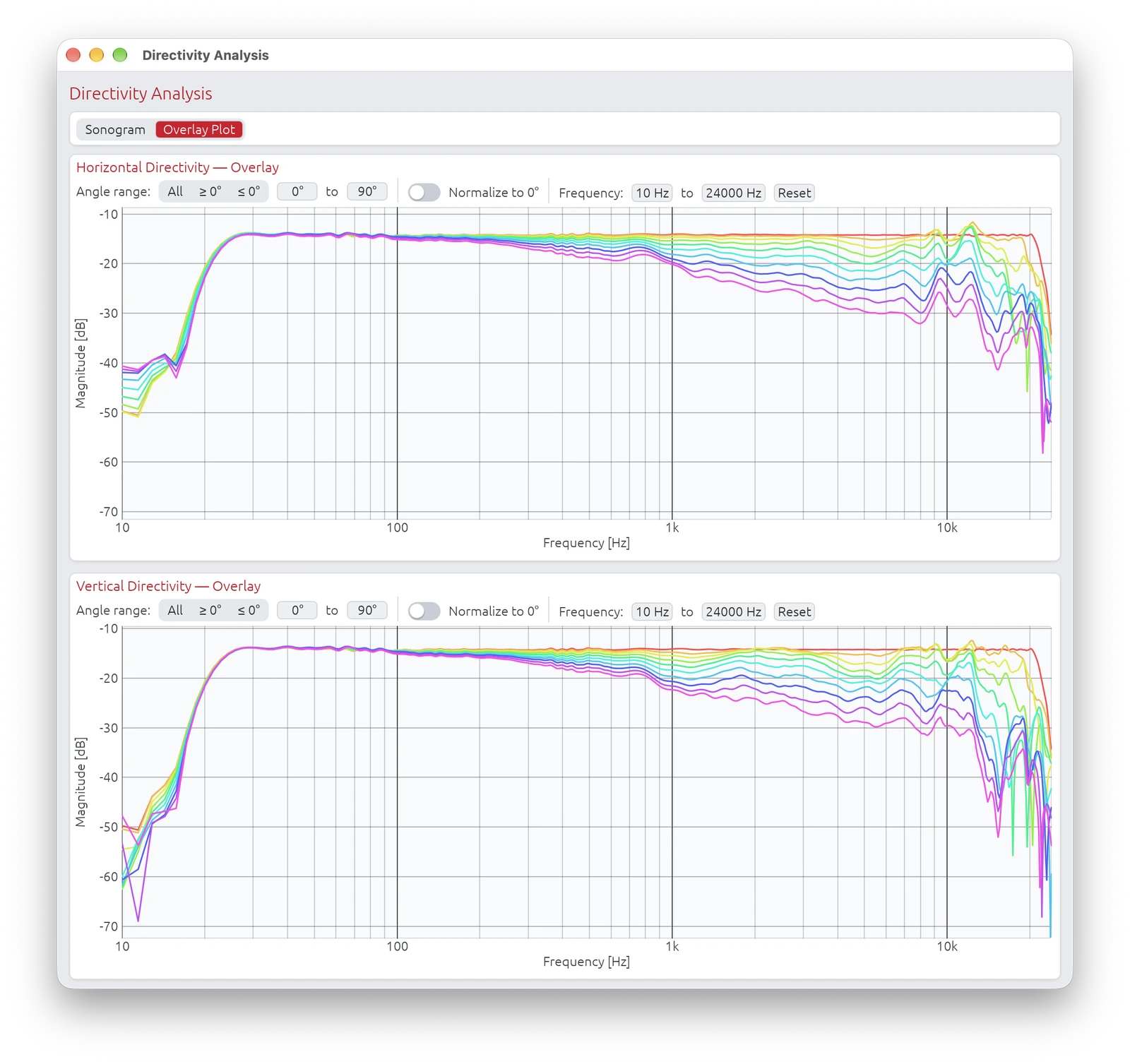
The Overlay Plot tab shows all measured off-axis frequency responses superimposed on a single graph, one coloured line per angle. It complements the sonogram by making it easier to read precise frequency-domain differences between angles.
Horizontal and vertical directivity are displayed one above the other, each with its own set of controls.
Curve Colours
Angles are mapped to a rainbow colour scale (red → yellow → green → cyan → blue → violet) from the minimum to the maximum angle in the current filter selection.
The angle, frequency, and magnitude are shown in a tooltip when hovering over a curve.
Angle Range Filter
Three preset buttons restrict which angles are plotted:
| Button | Effect |
|---|---|
| All | Show all measured angles |
| ≥ 0° | Positive angles only (0° to max) — default |
| ≤ 0° | Negative angles only (min to 0°) |
A drag-value min/max selector allows fine-grained control of the displayed range. The Y-axis auto-scale updates whenever the selection changes.
Normalize to 0°
The Normalize to 0° toggle divides each curve by the on-axis (0°) response (reference computed up to 20 kHz to avoid tweeter resonance peaks):
- The on-axis curve becomes flat at 0 dB
- All other curves show their deviation relative to on-axis at each frequency
- The Y-axis label changes to Relative Magnitude [dB]
- The vertical range is anchored to the configured magnitude lower bound (e.g. −30 dB to +3 dB)
- Curves can show positive dB values where the off-axis response exceeds the on-axis reference at a given frequency
Interpreting the Overlay Plot
Tightly clustered curves:
- Similar response at all angles → well-controlled directivity
- Especially important in the crossover region
Curves spreading at high frequencies:
- Normal behaviour — drivers beam as frequency rises
- A gradual, smooth spread indicates controlled directivity
Sudden divergence at a specific frequency:
- Possible crossover lobing or driver interference at that frequency
- Cross-reference with the sonogram to confirm
With Normalize to 0° enabled:
- Flat normalized curves (near 0 dB) across ±30° indicate a speaker whose tonal balance is consistent within the listening window
- A normalized curve that drops sharply above a certain frequency indicates the onset of beaming
- Positive dB values on off-axis curves indicate angles where the response exceeds the on-axis reference — this can occur with wider dispersion drivers or in crossover regions
Preserving Time-of-Flight
Each driver's measurements must keep their arrival time (their time-of-flight to the microphone), or the same offset removed from all of them: the interference between the drivers, which shapes the directivity, comes from these delays. Multi-Driver Interference explains why.
Proper Workflow
1. Capture IR with full time-of-flight intact
- Use proper timing reference (electric loopback or acoustic chirp)
- Do not apply windowing that removes acoustic delay
- Preserve the natural arrival time differences
2. Import into LinFIR preserving the delay
- Keep the raw impulse peak positions as captured or remove the same amount of time across all measurements
- Each angle will have slightly different delay values (this is correct)
3. Apply crossover filters
- Crossovers add their own phase shifts
- These combine with geometric delays
4. LinFIR predicts directivity
- Calculation includes both geometry (TOF) and filtering (crossover phase)
- CTA-2034-A power averages over the measured angles
- Result: realistic DI and sonograms
5. Sonogram shows realistic interference
- Interference patterns reflect both driver spacing and crossover design
- Allows optimization of crossover for desired directivity
Limitations and Best Practices
Measurement Density
More angle measurements = more accurate prediction
- Minimum recommended: 7 angles per axis (±90° in 30° steps)
- Good: 13 angles per axis (±90° in 15° steps)
- Ideal: 19 angles per axis (±90° in 10° steps) or finer
Why density matters:
- Sound Power and DI weight each measured angle by the part of the sphere it stands for: sparse angles sample the sphere coarsely and miss interference lobes between drivers
- CTA-2034-A measures both orbits all the way round in 10° steps (5° steps have standard weights too); Sound Power needs the rear half (±100° to 180°) as well, and the Rear Wall bounce 180° - without them the Sound Power only covers the front and comes out too high for a directional loudspeaker
- Fine measurements = more accurate directivity prediction
Room Reflections
Directivity analysis is most accurate in anechoic conditions
- Room reflections distort off-axis measurements
- Early reflections appear as interference in the sonogram
- Can create false lobing patterns
Mitigation strategies:
- Measure outdoors (less reflections)
- Measure in large room with speaker away from walls
- Use gating/windowing carefully:
- Remove late reflections (>10 ms after main arrival)
- Use Adaptive Window to preserve bass while gating reflections
Microphone Position
Keep measurement distance constant:
- Same distance for all angles
- Ensures consistent SPL normalization
- Eliminates distance-related level variations
Farfield measurements (>1 meter) work best:
- Avoids nearfield effects
- Drivers behave as coherent sound sources
- More accurate directivity prediction
- The results can then be calculated farther away (CTA-2034-A: 2 m) with the calculation distance; calculated closer than measured, the near field of large drivers is missing
Microphone height:
- Should match speaker acoustic center
- For 2-way speaker, typically between tweeter and woofer
- Ensures symmetric vertical measurements
Computational Notes
DI and the other spinorama curves:
- The drivers are summed at every measured angle, then the angles averaged at every frequency
- May take a few seconds for dense polar data
Sonogram generation:
- Creates high-resolution 2D images (frequency × angle)
- Parallel processing used for speed
- Results are cached to improve performance
Getting a License
To unlock Directivity Analysis tools:
- Visit the LinFIR website: https://demaudio.com/linfir/
- Purchase a license key
- Enter your e-mail and key in LinFIR: Settings → License
- All directivity features will be enabled immediately
Your license supports:
- Ongoing development
- New features
- Bug fixes and improvements
Related Documentation
- IR Management: Capturing and managing off-axis measurements
- Audio Setup: Configuring audio interface, measurement settings, and timing reference for accurate polar measurements
- Driver Processing: Crossover design and optimization
Summary
Directivity Analysis tools characterize how your speaker radiates sound in different directions:
Features:
- Off-axis frequency response visualization at any angle
- Directivity Index (DI) prediction across the spectrum
- Listening Window, Predicted In-Room Response (PIR), Early Reflections, Sound Power and Early Reflections DI curves, following the ANSI/CTA-2034-A ("CEA-2034") spinorama standard
- Directivity sonograms (2D colour-mapped heatmaps, frequency × angle)
- Overlay Plot (all off-axis curves superimposed, with angle range filter and normalize to 0° toggle)
Requirements:
- Valid LinFIR license
- Polar measurements at multiple angles (horizontal and vertical)
- Preserved time-of-flight
- Proper timing reference (electric loopback or acoustic chirp)
Key Concepts:
- Time-of-flight encodes driver geometry (must be preserved)
- DI quantifies how directional the speaker is (0 dB = omni, higher = more directional)
- Sonograms visualize radiation patterns (hot colors = on-axis energy, cool = off-axis attenuation)
- Overlay Plot superimposes all off-axis curves for precise frequency-domain comparison; normalize to 0° shows deviation relative to on-axis
- Crossover optimization based on directivity for consistent off-axis response
Workflow:
- Configure timing reference (electric loopback recommended)
- Capture polar measurements for each drivers (preserve time-of-flight)
- Design crossovers and apply filters
- View off-axis curves, DI, sonograms, and overlay plots
- Optimize crossover for desired directivity pattern
- Iterate based on measurements
Use directivity analysis to understand and optimize your speaker's radiation pattern for better room interaction and consistent sound across the listening area.