
The cascade of Hammerstein models, or parallel Hammerstein model, represents a nonlinear system as a sum of branches, each raising the input to a power and filtering it. Rébillat et al. proposed it to predict the harmonic distortion of electrodynamic loudspeakers [1]. It is also used to reproduce the nonlinearities of electronic circuits such as guitar overdrive pedals [2] and tube amplifiers [3].
Its filters, the kernels, can be estimated from a single exponential sweep, which measures the impulse response and the harmonic distortion in one go. That computation needs the phase of every harmonic response, and the textbook way to get the right phases is Novák's synchronized sweep. In its usual form, the one in the reference code of its authors, it does not let you choose the duration of the sweep freely.
This article is about estimating the kernels from an ordinary Farina sweep, left as it is. Its phase error is a constant for each harmonic order, which follows from the sweep's parameters. Removing it after the measurement gives the same kernels as the synchronized sweep, and it works on any Farina measurement, including old ones.
The short version:
- The response of order \(n\) of a Farina sweep is off by a constant phase, \(\varphi_c(n) = 2\pi f_1 L\,(n-1)\). Rotated back, a 5 s Farina sweep gives the kernels of a 46 s synchronized sweep, 0.018 dB and 0.08° apart in a simulation.
- Without the correction the kernels are wrong, magnitude included. In the same simulation, the error on the linear kernel was 3.5 %, and on the kernels of orders 3 to 5 it was larger than the kernels themselves.
- The usual synchronized sweep, which starts at phase zero, rounds its duration in steps of \(\ln(f_2/f_1)/f_1\). For a sweep starting at 0.25 Hz, two octaves below 1 Hz to leave room for a fade-in, the shortest one lasts 46 s.
- The only argument left for synchronizing is leakage between the harmonic windows when the sweep is very short. At equal duration, down to 0.1 s, I could not make it show.
1. From MLS to the exponential sweep
To measure an impulse response, you send a known signal through the system and undo it. For years the standard signal was the maximum-length sequence (MLS), a binary pseudo-random noise whose circular autocorrelation is almost a perfect impulse [4]. It is fast and copes well with background noise. Distortion, though, does not stay in one place. With a loudspeaker driven hard, it comes back as spurious peaks spread along the impulse response [5, 6].
Sweeps were not new. Heyser's time delay spectrometry used a linear sweep and a tracking filter as early as 1967 [7], and Aoshima's time-stretched pulse of 1981 is a sweep compressed back into an impulse by deconvolution [8]. In 2000, Farina proposed the exponential sweep, whose frequency grows by the same ratio every second [5]:
$$ x(t) = \sin\big(2\pi f_1 L\,(e^{t/L} - 1)\big), $$
where the sweep runs from \(f_1\) to \(f_2\) in \(T\) seconds and \(L = T/\ln(f_2/f_1)\) is the time it takes to multiply the frequency by \(e\). Its instantaneous frequency is \(f_1 e^{t/L}\).
The exponential sweep became the standard because of what it does with distortion. The \(n\)-th harmonic of the sweep reaches any given frequency \(L \ln n\) seconds before the sweep itself does. After deconvolution, the response of order \(n\) therefore lands \(L \ln n\) ahead of the linear impulse response, each order at its own place, and a window cuts it out. The idea of separating the harmonics with a sweep had appeared before, in papers by Craven and Gerzon [9] and by Griesinger [10], as Novák et al. point out [11]. For a 5 s sweep from 0.25 Hz to 24 kHz, \(L\) = 0.44 s. The second harmonic sits 0.30 s ahead of the impulse response, the third 0.48 s. Müller and Massarani later showed how much better sweeps cope with distortion and time variance than pseudo-noise signals [6].
2. From harmonic responses to kernels
Farina also wrote the system as a sum of branches, each raising the input to a power and filtering it [5]:
$$ y(t) = \sum_{n=1}^{N} g_n(t) * x^n(t). $$
This is the parallel Hammerstein model, the diagonal part of a Volterra series. Farina took the response found at the \(n\)-th place as the filter \(g_n\) of the \(n\)-th branch. The two are not the same thing, because a power of a sine contains several harmonics. \(x^3\) has a third harmonic, and also a component at the fundamental:
$$ \sin^3\phi = \tfrac{3}{4}\sin\phi - \tfrac{1}{4}\sin 3\phi. $$
The response measured at the place of order \(m\), call its spectrum \(H_m(f)\), is a mix of the kernels \(G_m\), \(G_{m+2}\), \(G_{m+4}\) and so on. Novák et al. [12] and Rébillat et al. [13] showed how to undo the mix with the identities that expand \(\sin^n\) into harmonics. At each frequency,
$$ H_m(f) = \sum_{n \ge m} a_{n,m}\, G_n(f), $$
with a triangular matrix of known coefficients, inverted frequency by frequency.
The coefficients are complex, because the even powers produce cosines: \(\sin^2\phi = \tfrac12 - \tfrac12\cos 2\phi\), and a cosine is a sine shifted by 90°. The inversion adds and subtracts complex spectra. If \(H_3\) comes with the wrong phase, \(G_1\) comes out wrong, magnitude included.
3. The phase problem, and Novák's synchronized sweep
For the inversion to work, the response at the place of order \(n\) must be exactly the \(n\)-th harmonic, with its phase. With the exponential sweep this rests on one identity. If \(\phi(t)\) is the phase of the sweep, delaying the sweep by \(L \ln n\) must give its \(n\)-th harmonic:
$$ n\,\phi(t) = \phi(t + L \ln n). $$
Farina's phase, \(\phi_F(t) = 2\pi f_1 L\,(e^{t/L} - 1)\), does not satisfy it. The culprit is the \(-1\), which is there to make the sweep start at phase zero. Novák et al. drop it [11]:
$$ \phi_N(t) = 2\pi f_1 L\, e^{t/L}, $$
which satisfies the identity for any \(L\). The sweep then starts at the phase \(2\pi f_1 L\) instead of zero, and the paper shows both versions [11]. To start at zero as well, they require \(f_1 L\) to be an integer \(k\), which is the version their reference code implements. The duration can no longer be anything:
$$ T = \frac{k \ln(f_2/f_1)}{f_1}, \quad k = 1, 2, 3, \ldots $$
Since \(k\) is an integer, \(T\), \(f_1\) and \(f_2\) are tied together, as the authors note [11].
4. The phase error of a Farina sweep is a constant
Compare the two sides of the identity with Farina's phase. The delayed sweep has the phase
$$ \phi_F(t + L \ln n) = 2\pi f_1 L\,(n\,e^{t/L} - 1), $$
and the \(n\)-th harmonic
$$ n\,\phi_F(t) = 2\pi f_1 L\,(n\,e^{t/L} - n). $$
Their difference does not depend on time:
$$ \varphi_c(n) = 2\pi f_1 L\,(n - 1). $$
The \(n\)-th harmonic of a Farina sweep is the delayed sweep rotated by \(-\varphi_c(n)\). A phase that is constant in time is the same phase at every frequency, so after deconvolution the response at the place of order \(n\) is the right one, multiplied by \(e^{-j\varphi_c(n)}\). The correction is to multiply it by \(e^{+j\varphi_c(n)}\), once the response has been cut out and aligned on its exact position. (Spectra are written with \(e^{-j2\pi ft}\). The rotation applies to the positive frequencies and its conjugate to the negative ones, which keeps the response real. In the time domain, it is a rotation of the analytic signal.)
For a 5 s sweep from 0.25 Hz to 24 kHz, \(f_1 L\) = 0.109 and the offsets of orders 2 to 5 are 39°, 78°, 118° and 157°. They change with every parameter of the sweep, and they are far from small.
To check this, I simulated a Hammerstein system of order 5. Its filters are arbitrary, shaped like a woofer's responses: a second-order high-pass between 30 and 70 Hz, a low-pass between 1 and 6 kHz, gains from 0 to −40 dB. The sweep runs from 0.25 Hz to 24 kHz at 48 kHz, with a fade-in over the first two octaves. The powers of the input are generated harmonic by harmonic and filtered as a converter would filter them, so nothing folds back below the Nyquist frequency. I measured the system with a 5 s Farina sweep and with Novák's sweep, which the integer condition stretched to 46 s.
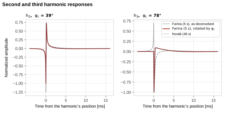
The rotated Farina responses lie on top of Novák's. As deconvolved, the third one, 78° off, does not even have the right shape.
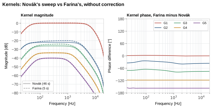
Without the correction, the error on the linear kernel \(G_1\) is 3.5 %, and on \(G_3\), \(G_4\) and \(G_5\) it is larger than the kernels themselves. \(G_4\) and \(G_5\) keep the right magnitude here, but their phase is off by \(\varphi_c\).
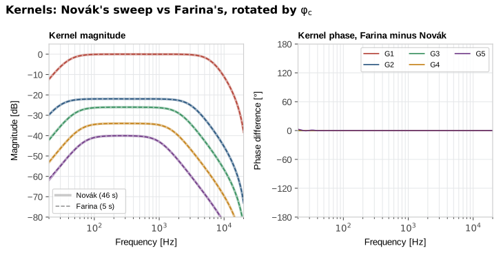
Corrected, the kernels of the 5 s Farina sweep match those of the 46 s synchronized sweep within 0.018 dB and 0.08° between 50 Hz and 5 kHz, and both match the exact kernels of the simulation.
The correction is not new. The toolbox of Schmitz and Embrechts, HKISS, which accompanies their work on Hammerstein kernels measured with a sine sweep, applies the same rotation to the harmonic responses of a Farina sweep [3].
5. What the synchronization costs
The integer condition rounds the duration in steps of \(\ln(f_2/f_1)/f_1\). The step depends mostly on the start frequency. With \(f_2\) = 24 kHz, it is 0.35 s for a sweep starting at 20 Hz, 1.7 s from 5 Hz and 10 s from 1 Hz.
A sweep meant to measure down to 1 Hz often starts two octaves lower, at 0.25 Hz, so that its fade-in is over before the band of interest. The step is then 46 s at 48 kHz, 49 s at 96 kHz. A synchronized 5 s sweep has to become a 46 s one, and the next durations available are 92 s and 138 s (97 s and 146 s at 96 kHz).
The other way out is to keep the duration and raise the start frequency. The lowest start for a synchronized 5 s sweep is 1.9 Hz, three octaves above 0.25 Hz, and for a 1 s sweep it is 8 Hz.
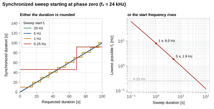
With the correction, \(T\), \(f_1\) and \(f_2\) are free, and \(\varphi_c(n)\) is computed from whatever they are.
Novák et al. also give a way out at the source. Without the integer condition, their sweep is synchronized at any duration and starts at the phase \(2\pi f_1 L\) [11]. Their reference code keeps the rounding, as do the toolboxes I looked at, and a measurement already made with a Farina sweep cannot be fixed that way.
6. When would a synchronized sweep still help?
The correction is applied after the harmonic responses have been cut out of the deconvolved signal. Before that, each Farina response is the true one rotated by \(-\varphi_c(n)\), which mixes in its Hilbert transform. The Hilbert transform of a short pulse is not short, it decays slowly on both sides of the peak. In principle, a rotated response spreads further in time, leaks into the windows of its neighbours and loses part of itself outside its own. The windows shrink as the sweep gets shorter and the order higher, since the gap between orders \(n\) and \(n+1\) is \(L \ln\frac{n+1}{n}\). Between orders 4 and 5 it is 97 ms for the 5 s sweep above, and less than 10 ms for a 0.5 s one.
To compare at equal duration, I use the synchronized sweep that starts at a non-zero phase, with a fade-in.
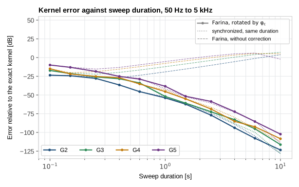
The corrected Farina sweep and the synchronized one stay together from 0.1 s to 10 s. Both lose accuracy as the sweep gets shorter, by the same amount, because the system's own responses are a few tens of milliseconds long and no longer fit in windows of a few milliseconds. The rotation adds nothing visible on top of that.
The leakage exists on paper, but I could not make it show. And with the integer condition, the comparison is not even at equal duration. Synchronizing a sweep from 0.25 Hz stretches it from 5 s to 46 s, and in a 46 s sweep the fourth and fifth harmonics are 0.9 s apart.
If you want the harmonic responses in their true shape before any windowing, for instance to look at the raw deconvolved signal, that sweep gives it at any duration. Both routes lead to the same kernels, and the correction leaves the sweep untouched.
Author's note. The figures come from a simulated Hammerstein system of order 5, without noise, so that the comparison is between the sweeps alone. The correction is in the toolbox of Schmitz and Embrechts [3], yet it is rarely mentioned. Novák et al. show the phase errors of a non-synchronized sweep on a woofer and remove them by synchronizing the sweep [11], and at least one recent toolbox documents the harmonic phases of a Farina sweep as unusable. If you know of an earlier source, write to me and I will cite it.
References
Rébillat, M., Hennequin, R., Corteel, É. and Katz, B. F. G., "Prediction of harmonic distortion generated by electro-dynamic loudspeakers using cascade of Hammerstein models", 128th AES Convention, London, 2010.
Novák, A., Simon, L. and Lotton, P., "Analysis, synthesis, and classification of nonlinear systems using synchronized swept-sine method for audio effects", EURASIP Journal on Advances in Signal Processing, 2010, 793816. Two guitar overdrive pedals.
Schmitz, T. and Embrechts, J.-J., "Hammerstein kernels identification by means of a sine sweep technique applied to nonlinear audio devices emulation", Journal of the Audio Engineering Society, 65(9), 696–710, 2017. An overdrive effect and two tube amplifiers. Their Matlab toolbox, HKISS, multiplies the response of order \(k\) by \(e^{j(k-1)\,2\pi f_1 L}\) (
computeKernel.m).Rife, D. D. and Vanderkooy, J., "Transfer-function measurement with maximum-length sequences", Journal of the Audio Engineering Society, 37(6), 419–444, 1989.
Farina, A., "Simultaneous measurement of impulse response and distortion with a swept-sine technique", 108th AES Convention, Paris, preprint 5093, 2000. The exponential sweep.
Müller, S. and Massarani, P., "Transfer-function measurement with sweeps", Journal of the Audio Engineering Society, 49(6), 443–471, 2001.
Heyser, R. C., "Acoustical measurements by time delay spectrometry", Journal of the Audio Engineering Society, 15(4), 370–382, 1967.
Aoshima, N., "Computer-generated pulse signal applied for sound measurement", Journal of the Acoustical Society of America, 69(5), 1484–1488, 1981. The time-stretched pulse.
Craven, P. G. and Gerzon, M. A., "Practical adaptive room and loudspeaker equaliser for hi-fi use", AES UK 7th Conference: Digital Signal Processing, 1992.
Griesinger, D., "Beyond MLS: occupied hall measurement with FFT techniques", 101st AES Convention, 1996.
Novák, A., Lotton, P. and Simon, L., "Synchronized swept-sine: theory, application, and implementation", Journal of the Audio Engineering Society, 63(10), 786–798, 2015. The synchronized sweep, with and without a zero starting phase (eqs. 28 and 33), and the phase errors of a non-synchronized sweep on a woofer (Fig. 7).
Novák, A., Simon, L., Kadlec, F. and Lotton, P., "Nonlinear system identification using exponential swept-sine signal", IEEE Transactions on Instrumentation and Measurement, 59(8), 2220–2229, 2010.
Rébillat, M., Hennequin, R., Corteel, É. and Katz, B. F. G., "Identification of cascade of Hammerstein models for the description of nonlinearities in vibrating devices", Journal of Sound and Vibration, 330(5), 1018–1038, 2011.