The dB Wars: Commentary on an Impossible Specification
June 2026 — Arnaud Demion
In early 2026, a professional loudspeaker manufacturer announced its new large-format touring system. The product datasheet, picked up by several trade publications, displayed two figures side by side:
- Max SPL: 160 dB (Peak)
- Frequency range: 35 Hz – 20 kHz
Those two numbers stopped me cold.
Taken individually, each can be read as a plausible extrapolation of market trends — the industry has been engaged in a peak SPL escalation for years, and every product generation outbids its predecessor. Taken together, however, they create a fundamental problem: they are not consistent with the laws of physics.
This article is based on the technical memorandum I submitted to the AES (Audio Engineering Society), addressed to Subcommittee SC-04. The reasoning is entirely general — it applies to any system publishing comparable figures without disclosing measurement conditions.
A note on intent. This article is an exercise in technical commentary, not an accusation. The analysis examines publicly available specifications against standard physical models — nothing more, nothing less. If any manufacturer can point to a measurement protocol, a theoretical framework, or any information that I may have overlooked, which renders the claimed figures physically achievable, I invite the reader to provide it. I am not claiming to have the final word. I am claiming only that, based on the information available to me, the numbers as stated cannot be reconciled with established physics. The burden of proof, I would argue, lies with whoever publishes them, and that is precisely why this document exists: to contribute, however imperfectly, to a conversation that the industry urgently needs.
1. What the specification implies
In professional practice, Max SPL is used as the anchor for inverse-square-law propagation calculations:
$$\text{SPL}(r) = \text{SPL}_{1\ \text{m}} - 20\log_{10}(r)$$
A sound engineer who accepts 160 dB at 1 m will predict 140 dB at 10 m and 126 dB at 50 m. If the physical reality is closer to 135 dB — as we will show — those predictions become 115 dB and 101 dB. A 25 dB error across the entire coverage area.
The equivalent would be calculating that ten thousand spectators fit in a venue that physically holds sixteen.
The impossibility of comparison
For the acoustician, specifications of this form are not engineering data, they are unverifiable claims. They cannot be compared with one another because none is anchored to a measurement protocol or a reproducible theoretical calculation. What we observe is a race in which manufacturers seem to compete in publishing ever more ambitious technical figures, figures that increasingly exceed the limits of linear acoustics.
As this document demonstrates, we are unable — from a theoretical standpoint and under the most favourable assumptions — to recover the announced figures on the basis of the available information alone. I invite anyone who can demonstrate otherwise to provide any measurement protocol, any theoretical model, or any piece of information that may have escaped this analysis, which would render the claimed figures physically achievable. The analysis below proceeds on the generous assumption that they are, and shows that even under that assumption, the numbers remain out of reach.
2. A first sanity check: required amplifier power
Before any detailed physics, a back-of-the-envelope calculation is enough to raise a red flag. A professional woofer or subwoofer driver typically achieves a sensitivity of 95–98 dB SPL at 1 m for 1 W of input — 100 dB would already be considered generous for a low-frequency transducer. The relationship between sensitivity, power, and on-axis SPL is:
$$\text{SPL}(1\ \text{m}) = S + 10\log_{10}(P)$$
where \(S\) is the sensitivity in dB/W/m and \(P\) is the electrical input power in watts. Taking \(S = 98\) dB as a generous upper bound, the power required to reach 160 dB at 1 m is:
$$P = 10^{(160 - 98)/10} = 10^{6.2} \approx \mathbf{1.6\ \text{MW}}$$
With the more typical \(S = 95\) dB, the figure rises to \(10^{6.5} \approx 3.2\) MW.
One to three megawatts. From a single enclosure.
This figure alone should terminate any engineering conversation about 160 dB at 1 m as a meaningful, usable specification. It does have well-known limits as a rigorous argument: it treats the cabinet as a single uncoupled driver, ignores mutual coupling between multiple transducers, and does not account for directivity. A more rigorous approach is required. The two sections below develop independent physical bounds — one from mechanical displacement, one from nonlinear acoustics — that do not rely on sensitivity figures and yield the same qualitative conclusion.
3. Second bound: mechanical displacement
The target pressure
160 dB (Peak) corresponds to a peak acoustic pressure of:
$$p_\text{peak} = 20 \times 10^{-6} \times 10^{160/20} = 2000 \text{ Pa}$$
Approximately 2.0% of atmospheric pressure. We will return to that.
The source radiates as a compact piston at 35 Hz
At 35 Hz the wavelength in air is \(\lambda = c/f \approx 9.8\) m. Since all cabinet dimensions are much smaller than \(\lambda\), the system behaves as a compact piston source (\(ka \ll 1\) at 35 Hz: \(ka \approx 0.15\) for an 18-inch driver). In this regime the source radiates as a point monopole, and the monopole pressure formula holds exactly at all distances \(r > a\) — there is no near-field amplitude correction.
The monopole radiation equation in half-space can be derived from first principles. For a cone executing sinusoidal displacement \(x(t) = x_0\sin\omega t\), the velocity and acceleration follow by differentiation:
$$\begin{aligned} v(t) &= \omega\ x_0\cos(\omega t) \\ a(t) &= -\omega^2\ x_0\sin(\omega t) \end{aligned}$$
The radiated pressure is proportional to cone acceleration. In half-space (\(2\pi\) sr, infinite-baffle condition) the peak pressure at distance \(r\) is:
$$p_\text{peak} = \frac{\rho_0\ S_d}{2\pi r}\ a_\text{peak} = \frac{\rho_0\ S_d}{2\pi r}\ \omega^2\ x_0 = \frac{\rho_0\ \omega^2\ V_{d,\text{peak}}}{2\pi r}$$
where \(V_{d,\text{peak}} = S_d \cdot x_0\) is the peak volume displacement, \(\rho_0 = 1.225\) kg/m³, \(\omega = 2\pi \times 35 \approx 219.9\) s⁻¹, so \(\omega^2 \approx 48{,}361\) s⁻². The denominator \(2\pi r\) (half-space) rather than \(4\pi r\) (free space) already represents the most favourable possible assumption: it supposes that all acoustic energy is radiated into the forward hemisphere only, yielding a pressure double that of the free-space case.
Solving for the required volume displacement at \(r = 1\) m:
$$V_{d,\text{peak}} = \frac{p_\text{peak} \cdot 2\pi r}{\rho_0\ \omega^2} = \frac{2000 \times 2\pi \times 1}{1.225 \times 48{,}361} \approx \mathbf{0.212\ \text{m}^3}$$
Transducer architecture
The cabinet in question houses four 15-inch drivers and two 18-inch drivers mounted laterally for cardioid bass control. Typical effective diaphragm areas for professional high-excursion drivers of these sizes are:
| Driver | \(S_d\) (m²) | Count |
|---|---|---|
| 15-inch | 0.0855 | 4 |
| 18-inch | 0.123 | 2 |
Assuming perfect in-phase coupling of all drivers — a deliberately over-generous hypothesis:
$$S_{d,\text{total}} = 4 \times 0.0855 + 2 \times 0.123 = 0.588 \text{ m}^2$$
Note on the cardioid configuration. In a cardioid bass system, the lateral drivers do not contribute to the net forward volume velocity: their function is to cancel rearward radiation by providing the dipole term. The effective area \(S_{d,\text{total}}\) above is therefore already a strict upper bound — the physical reality is less favourable. Furthermore, no practical cardioid achieves infinite rear attenuation: rear rejection is typically 15–20 dB in professional implementations, meaning a non-negligible fraction of the lateral drivers’ motion is simply lost as rearward radiation.
The required peak excursion per driver becomes:
$$X_\text{peak} = \frac{0.212}{0.588} \approx 360 \text{ mm}$$
Mechanical limit. State-of-the-art professional high-excursion drivers in the 15–18-inch class typically achieve a linear peak excursion (\(X_\text{max}\)) of 15–20 mm, with a mechanical travel limit of approximately 25 mm. The 360 mm required exceeds this limit by a factor greater than 15.
Physically achievable SPL at 35 Hz
Using the best-case parameters — \(X_\text{peak} = 20\) mm, \(S_{d,\text{total}} = 0.588\) m²:
$$p_\text{max} = \frac{1.225 \times (2\pi \times 35)^2 \times 0.588 \times 0.020}{2\pi} \approx 111 \text{ Pa}$$
$$\text{SPL}_\text{max} = 20\log_{10}\left(\frac{111}{20 \times 10^{-6}}\right) \approx 135 \text{ dB SPL (Peak)}$$
The gap between the claimed figure and the physical maximum is therefore:
$$\Delta SPL = 160 - 135 = \mathbf{25\ \text{dB}}$$
corresponding to a factor of \(10^{25/10} \approx 316\) in acoustic power. No realistic combination of measurement uncertainty, coupling efficiency, or near-field correction can account for a discrepancy of this magnitude.
A charitable bound: the bass-reflex port contribution
The cabinet in question is a bass-reflex design. At the tuning frequency, the port radiates in phase with the cone and contributes additively to the total volume velocity. We account for this contribution explicitly rather than treating the cone as the sole radiator.
An already generous starting assumption. The calculation below assumes the cone is driven at its full best-case excursion ($X_\mathrm{peak} = 20$ mm) simultaneously with the port operating at its own limit. In a real bass-reflex system near $f_b$, the cone is significantly unloaded by the port and does not in fact need to reach $X_\mathrm{max}$ to contribute its share — meaning a real system would have even less cone output available than assumed here, not more. Granting full $X_\mathrm{max}$ to the cone in addition to a generous port is therefore already charitable beyond normal operating conditions, not a realistic operating point.
Combined volume velocity. For the cone, executing sinusoidal displacement with peak amplitude $X_\mathrm{peak}$, the peak velocity is $\omega X_\mathrm{peak}$, so the total peak volume velocity is: $$ U_\mathrm{total} = U_\mathrm{cone} + U_\mathrm{port} = \omega S_d X_\mathrm{peak} + S_p v_p $$ We adopt $f_b = 40$ Hz and retain $S_{d,\mathrm{total}} = 0.588\ \mathrm{m^2}$, $X_\mathrm{peak} = 20$ mm: $$ U_\mathrm{cone,max} = \omega S_{d,\mathrm{total}} X_\mathrm{peak} = 2\pi \times 40 \times 0.588 \times 0.020 \approx 2.96\ \mathrm{m^3/s} $$ corresponding to 137.2 dB (Peak) from the cone alone — consistent with the increased radiation efficiency at 40 Hz compared to the 135 dB obtained at 35 Hz.
Total volume velocity required for 160 dB at 40 Hz, 1 m: $$ U_\mathrm{total,required} = \frac{p_\mathrm{peak}\cdot 2\pi r}{\rho_0\omega} = \frac{2000 \cdot 2\pi}{1.225 \times 2\pi \times 40} = \frac{2000}{1.225 \times 40} \approx 40.8\ \mathrm{m^3/s} $$ Crediting the cone’s full best-case contribution, the port alone must supply the remainder: $$ U_\mathrm{port,required} = U_\mathrm{total,required} - U_\mathrm{cone,max} \approx 37.8\ \mathrm{m^3/s} $$
Calculation 1 — port area required to stay below a given flow-speed ceiling. Flow velocities are used here purely as a comparative yardstick, not as a precise turbulence threshold; the qualitative picture is the same regardless of where exactly the line is drawn:
| Ceiling | Port velocity | Required port area $S_p$ |
|---|---|---|
| Mach 0.15 | 51.4 m/s | 0.74 m² |
| Mach 0.20 | 68.6 m/s | 0.55 m² |
Both required areas exceed $S_{d,\mathrm{total}} = 0.588\ \mathrm{m^2}$ and the Mach 0.15 figure probably exceeds the front face of the cabinet relative to what remains once the drivers themselves are accounted for. Even granting a flow speed considered fast by any standard, the port footprint required is incompatible with a cabinet that must also house six drivers, a midrange section, and an HF horn.
Calculation 2 — required flow velocity for a generously sized, realistic port. With the port area set equal to the entire driver complement, $S_p = S_{d,\mathrm{total}} = 0.588\ \mathrm{m^2}$ — already a generous allocation — what velocity would the port air need to reach? $$ v_\mathrm{port,required} = \frac{U_\mathrm{port,required}}{S_p} = \frac{37.8}{0.588} \approx \mathbf{64\ m/s} \approx \mathbf{Mach\ 0.187} $$ At this velocity, the dynamic pressure associated with the flow is: $$ \Delta p_\mathrm{dyn} = \tfrac12 \rho_0 v^2 \approx 2{,}500\ \mathrm{Pa} $$ roughly equal to the target acoustic peak pressure (2,000 Pa). At this point the port’s behaviour is governed by flow separation and turbulent loss rather than the linear radiation model the entire calculation depends on; the port stops acting as an efficient radiator well before reaching the required output.
Summary
| Configuration | Volume velocity (m³/s) | Outcome |
|---|---|---|
| Cone only, $X_\mathrm{max} = 20$ mm | 2.96 | 137.2 dB (Peak) |
| Port area required at Mach 0.15 | 37.8 | $S_p \approx 0.74\ \mathrm{m^2}$ — exceeds total driver area, approaches cabinet front face |
| Port area required at Mach 0.20 | 37.8 | $S_p \approx 0.55\ \mathrm{m^2}$ — roughly equal to total $S_d$ |
| Port velocity required at $S_p = S_{d,\mathrm{total}}$ | 37.8 | $v \approx 64\ \mathrm{m/s}$, Mach 0.187 — flow regime where the linear model breaks down |
Both directions of the calculation converge on the same conclusion. A port large enough to stay within a comfortable flow regime is larger than the cabinet can accommodate alongside its drivers. A port small enough to fit alongside the drivers must move air fast enough that the dynamic pressure of the flow itself rivals the target acoustic pressure, at which point the assumption of efficient linear radiation no longer holds. The bass-reflex port does not close the gap to the claimed 160 dB under any allocation of cabinet volume consistent with also housing six bass drivers, a midrange section, and a coaxial HF horn within a \(\approx 1000.0\) liters enclosure.
A bass-reflex port cannot bridge the gap. One might argue that exotic bass reflex alignments could theoretically increase the loudspeakers’ gain. Even granting that an optimised alignment could push the port contribution to +10 dB or more — a generous hypothesis that already pushes the design far from any practical operating point — the mechanically limited cone output at 35-40 Hz caps the total at roughly 145 dB Peak. The 15 dB shortfall from 160 dB remains. A bass-reflex port, no matter how cleverly aligned, cannot compensate for the 25 dB gap between the claimed figure and the physical maximum at 35 Hz.
4. Third bound: nonlinear acoustics
Even if the mechanical limitation were somehow overcome, a second physical barrier would prevent the stated performance.
Governing equations
Wave propagation at such amplitudes (≈ 2.0% of \(P_\text{atm}\)) is governed not by the linear wave equation but by the Burgers equation [1]:
$$\frac{\partial p}{\partial x} - \frac{\beta}{\rho_0 c_0^3}\ p\ \frac{\partial p}{\partial \tau} = \frac{\delta}{2\rho_0 c_0^3}\ \frac{\partial^2 p}{\partial \tau^2}$$
where \(\beta = 1 + B/(2A) \approx 1.2\) is the coefficient of nonlinearity of air, \(\tau\) is the retarded time, and \(\delta\) is the thermoviscous diffusivity. The nonlinear term causes progressive steepening of the waveform toward a sawtooth shock profile, transferring energy from the fundamental to higher harmonics and dissipating it thermally.
For a directional source such as a line array, the KZK equation (Kuznetsov–Zabolotskaya–Khokhlov) additionally accounts for diffraction:
$$\frac{\partial}{\partial \tau}\left[\frac{\partial p}{\partial x} - \frac{\beta}{\rho_0 c_0^3}\ p\ \frac{\partial p}{\partial \tau} - \frac{\delta}{2\rho_0 c_0^3}\ \frac{\partial^2 p}{\partial \tau^2}\right] = \frac{c_0}{2}\ \nabla_\perp^2\ p$$
Why the wave steepens: local sound speed variation
At small amplitudes, the adiabatic equation of state \(p \propto \rho^\gamma\) is linearised around the equilibrium: the sound speed \(c_0 = \sqrt{\gamma P_0 / \rho_0}\) is treated as constant, and the linear wave equation is exact. For pressures of 2,000 Pa — 2.0% of atmospheric pressure — this linearisation breaks down. Retaining the next-order term of the equation of state yields a pressure-dependent local sound speed:
\[c_\text{local} \approx c_0 + \beta\ u\]
where \(u\) is the local particle velocity and \(\beta \approx 1.2\) for air. This single correction is the physical origin of all the nonlinear effects described here.
The consequence is direct: compressive half-cycles travel slightly faster than \(c_0\); rarefaction half-cycles travel slightly slower. The leading edge of each positive pressure peak catches up with the preceding trough; the waveform progressively leans forward. The mathematics is identical to that of ocean waves approaching a beach: the crest, where the water column is tallest and the wave speed highest, advances faster than the trough — until the wave breaks.
The figure below illustrates this evolution for a single sinusoidal cycle. The normalised distance \(\sigma = x / l_\text{shock}\) is the implicit parameter of the exact solution of the lossless Burgers equation:
\[P = \sin(\theta + \sigma\ P)\]
where \(P = p / p_\text{max}\) and \(\theta = \omega\tau\) is the retarded phase ([1] §2.3, [2] §2.8). At \(\sigma = 0\) the waveform is a pure sine; at \(\sigma = 1\) the front develops a vertical slope — a pressure discontinuity.
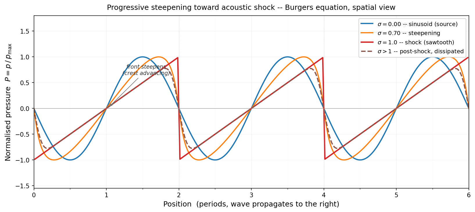
Progressive steepening of a sinusoidal wave toward a sawtooth shock profile. \(\sigma = x / l_\text{shock}\) increases from 0 (pure sine) to 1 (sawtooth). Post-shock (dashed): thermoviscous dissipation blunts the sawtooth teeth.
Harmonic redistribution. The shocked sawtooth has a specific Fourier spectrum: the amplitude of the \(n\)-th harmonic is proportional to \(1/n\). A 1 kHz tone that shocks before reaching the audience therefore arrives with strong energy at 2 kHz, 3 kHz, 4 kHz, … — a spectral signature indistinguishable from that of a hard-clipping amplifier. This distortion is a property of the propagating medium, not of the transducer or amplifier.
Thermoviscous dissipation. The \(\delta\) term on the right-hand side of the Burgers equation is a second-order temporal derivative; it therefore acts as a quadratic low-pass filter on the harmonic series — attenuation grows as \(n^2\). The sharp sawtooth teeth are progressively blunted: the wave transitions from a sharp sawtooth to a rounded (“old-age”) profile and eventually to a smooth wave of reduced amplitude. The acoustic energy is not recovered: it is converted to heat in the medium within a few metres of the source.
Shock formation distance — plane wave and diverging wave
For a plane sinusoidal wave, the Earnshaw solution gives the shock formation distance [1]:
$$l_\text{plane} = \frac{\rho_0\ c_0^3}{\beta\ \omega\ p_0} = \frac{\rho_0\ c_0^3}{2\pi f\ \beta\ p_0}$$
The Earnshaw formula is strictly valid for constant-amplitude plane waves. For a real loudspeaker, amplitude decays as \(p(r) = p_0(r_0/r)^\alpha\) with \(r_0 = 1\) m. Integrating the nonlinear phase accumulation along the propagation path [1]:
$$\int_{r_0}^{r_\text{shock}} \frac{\beta\ \omega\ p_0}{\rho_0 c_0^3} \left(\frac{r_0}{r}\right)^\alpha dr = 1$$
yields, for \(\alpha \neq 1\):
$$r_\text{shock} = r_0\left(1 + (1-\alpha)\ \frac{l_\text{plane}}{r_0}\right)^{1/(1-\alpha)}$$
and in the spherical limit \(\alpha \to 1\):
$$r_\text{shock}^\text{(sph)} = r_0\exp\left(\frac{l_\text{plane}}{r_0}\right)$$
The three relevant geometries are:
- \(\alpha = 0\): plane wave — the Earnshaw lower bound;
- \(\alpha = 1/2\): cylindrical spreading — appropriate for a line array operating in its intended throw range, where on-axis pressure decays as \(1/\sqrt{r}\);
- \(\alpha = 1\): spherical spreading — the most favourable possible bound, corresponding to the far field of a point source.
When \(l_\text{plane} \ll r_0\), all three expressions converge: the divergence correction becomes negligible and the shock always forms close to the reference distance.
The table below gives numerical results at both 160 dB and 140 dB (Peak):
| Frequency | 160 dB — plane | 160 dB — cyl. | 140 dB — plane | 140 dB — cyl. |
|---|---|---|---|---|
| 35 Hz | 95 m | No shock | 938 m | No shock |
| 100 Hz | 34 m | 302 m | 329 m | No shock |
| 500 Hz | 7.6 m | 18 m | 67 m | No shock |
| 1 kHz | 4.3 m | 7.0 m | 34 m | 303 m |
| 5 kHz | 1.7 m | 1.8 m | 7.5 m | 18 m |
| 10 kHz | 1.3 m | 1.3 m | 4.3 m | 7.0 m |
| 20 kHz | 1.2 m | 1.2 m | 2.6 m | 3.3 m |
Shock formation distance for plane wave and cylindrical divergence (\(\alpha=1/2\), appropriate for a line array). Reference distance \(r_0 = 1\) m. The spherical bound (\(\alpha=1\)) lies above the cylindrical values and is shown in the figure below.
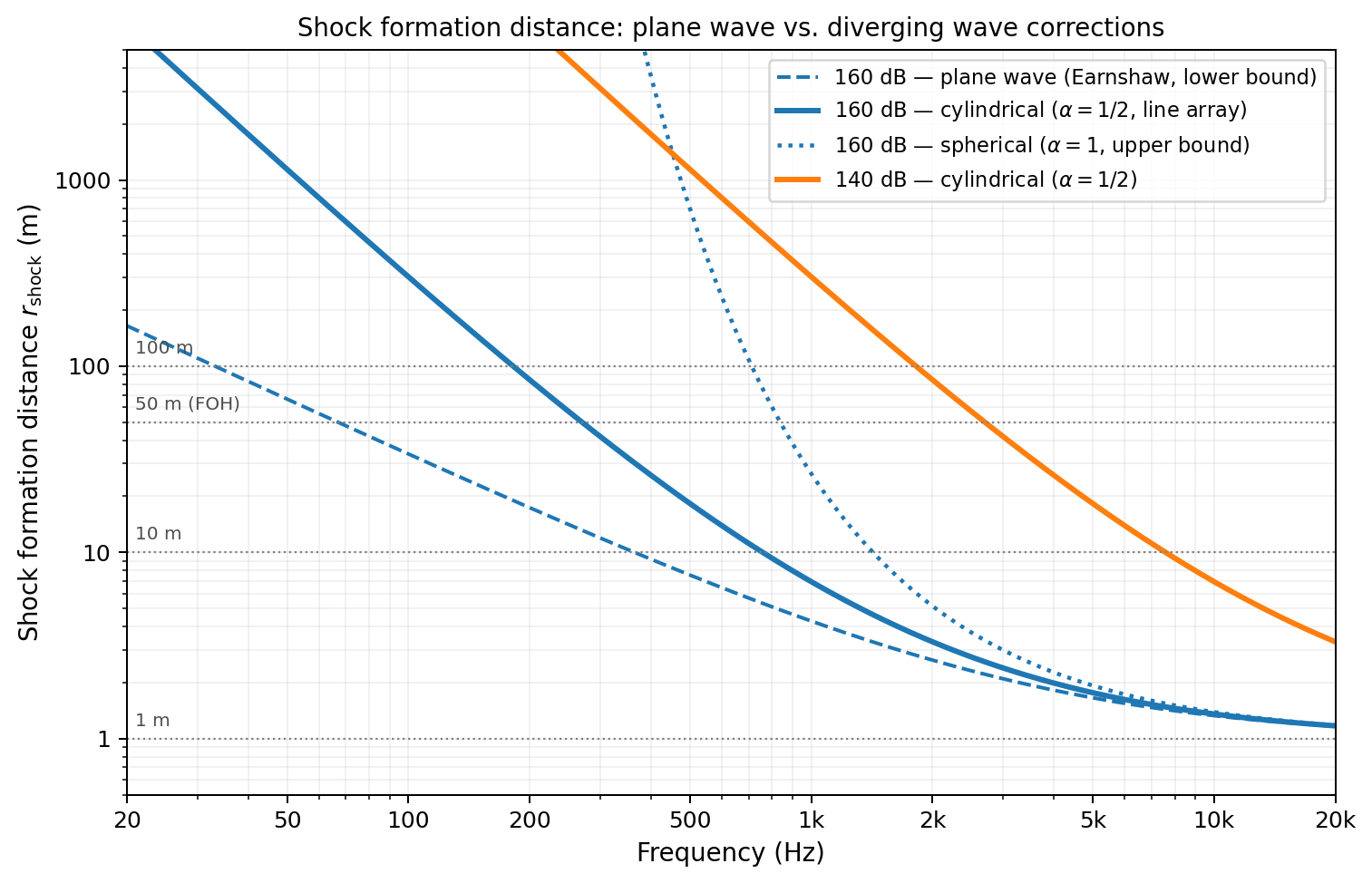
Shock formation distance at 160 dB and 140 dB (Peak), comparing three propagation geometries: plane wave (dashed), cylindrical (\(\alpha=1/2\), solid), and spherical (\(\alpha=1\), dotted — most favourable bound). At frequencies above 5 kHz all three models converge, as \(l_\text{plane}/r_0 < 0.5\).
Consequences for sound quality
Beyond the shock formation distance, a sinusoidal source component can no longer be treated as a single-frequency tone: the waveform has steepened into a sawtooth profile, and energy is continuously redistributed from the fundamental toward all odd and even harmonics. The amplitude of the \(n\)-th harmonic grows as \(1/n\) in the fully shocked regime — a spectral signature indistinguishable from that of a severely clipping amplifier. This distortion is imposed by the thermodynamic properties of air and cannot be corrected by any signal processing upstream.
At 160 dB, using the cylindrical model appropriate for a line array:
- Above 5 kHz: \(l_\text{plane}/r_0 \leq 0.5\), all three models converge to \(r_\text{shock} \approx 1.5\) m. The wave shocks within arm’s reach of the cabinet face regardless of geometry.
- At 1 kHz: \(r_\text{shock} \approx 7.0\) m (cylindrical), \(\approx 27\) m (spherical). Both are within or at the front rows of any concert audience.
- At 500 Hz: \(r_\text{shock} \approx 18\) m (cylindrical), \(\approx 709\) m (spherical). The two models diverge significantly; the cylindrical estimate corresponds to stage proximity.
- Below 100 Hz: the cylindrical model pushes \(r_\text{shock}\) well beyond any practical audience distance. This is also the frequency range where the mechanical displacement argument already excludes the stated performance.
Nonlinearity at 140 dB: a charitable lower bound
One might argue that the 160 dB figure applies only at the measurement point, and that a realistic deployment operates at lower levels. At 140 dB (Peak) — 20 dB below the claimed maximum, a factor of 100 in acoustic power — with cylindrical spreading:
- Below 100 Hz: \(r_\text{shock} \gg 1\) km — no nonlinear issue.
- At 1 kHz: \(r_\text{shock} \approx 303\) m. Transient and harmonic distortion is negligible up to and including the front of house (FOH) position.
- At 5 kHz: \(r_\text{shock} \approx 18\) m. High-frequency overtones, consonants, and transients are distorted before reaching the first rows of any large venue.
- At 10 kHz: \(r_\text{shock} \approx 7.0\) m. Distortion of treble content occurs at the edge of the stage area.
On the economic argument
The standard commercial pitch for a very high peak SPL figure is straightforward: “fewer boxes to cover the same venue — less trucking, less rigging, less cost.” This argument does not address nonlinearity, and it raises two additional problems.
First, fewer sources impair directivity control. A line array achieves its defining propagation behaviour — a cylindrical wave front with controlled vertical directivity — only when its aperture is sufficiently large relative to the wavelength at the frequencies of interest. Reducing the number of enclosures shortens the physical aperture, narrows the frequency range over which the array behaves as a coherent radiator, and increases the risk of grating lobes and uncontrolled spill. The array length is a degree of freedom that cannot be traded away for cost without direct consequences on the acoustic result.
Second, concentrating acoustic power on fewer sources makes the nonlinearity problem worse, not better. If the same total sound power must be delivered to the audience but is distributed across half as many enclosures, each cabinet must radiate twice the acoustic power, raising its near-field pressure by approximately +6 dB. Since \(l_\text{shock} \propto 1/p_0\), the shock formation distance is halved for every 6 dB increase in source pressure. Source concentration is precisely the condition that brings the propagating medium closest to the shock threshold.
Medium-limited fidelity. Assuming a hypothetically perfect, distortion-free transducer system capable of producing 160 dB (Peak) over the full 35 Hz–20 kHz bandwidth, the propagating medium would still impose catastrophic harmonic distortion at all mid- and high-frequency components before the wave reached any realistic listener position. A sound engineer accepting these specifications at face value would not only be working with a systematically wrong coverage model, but would also be unaware that the reproduced content above a few hundred hertz would be fundamentally compromised — by physics, not by equipment failure.
5. The absence of measurement conditions
The most fundamental question may not be “is this physically possible?” but “under what conditions was this figure measured?”
A Max SPL specification without the following information is not engineering data:
- Measurement distance (typically 1 m by convention, but never stated)
- Signal type (pink noise, sine tone, burst, shaped stimulus)
- Time window (a 5 ms burst tolerates a mechanically impossible sustained excursion)
- Spatial configuration (half-space, free field, room, outdoor)
- Frequency or frequency band to which the figure applies
Without this information, the value is:
- Non-verifiable by any independent third party,
- Non-comparable with data from a manufacturer who does specify conditions,
- Operationally misleading to any engineer using it as the anchor of a coverage calculation.
This is not a problem unique to this manufacturer. The absence of a mandatory disclosure standard for Max SPL measurement conditions in professional audio has produced a structural numbers war: manufacturers who publish conservative, fully qualified specifications are systematically disadvantaged in competitive tenders against those who do not. This is precisely the lemon market dynamic described by Akerlof in 1970 [3]: information asymmetry progressively drives quality out of the market.
6. Summary
| Parameter | Value |
|---|---|
| Claimed Max SPL | 160 dB (Peak) |
| Claimed lower bandwidth limit | 35 Hz |
| Required peak excursion at 35 Hz for 160 dB at 1 m | 360 mm |
| Maximum achievable peak excursion (best-case drivers) | ≈ 20 mm |
| Physically achievable Max SPL at 35 Hz (with optimistic BR) | ≈ 145 dB (Peak) |
| Discrepancy | 15 dB (factor 16 in power) |
Conclusion: the missing standard
I submitted this memorandum to AES SC-04 with a simple request: initiate or accelerate work on a mandatory disclosure standard for SPL measurement conditions in professional loudspeaker product literature — along the lines of what already exists for studio monitors ([4], [5]).
The objective is not to single out one manufacturer, but to establish a level playing field in which engineering claims are verifiable, comparable, and traceable to physical reality. The professional audio industry is technically sophisticated. Its engineers deserve data that is too.
A final invitation. I have laid out my analysis here in the hope that someone, somewhere, can show me where I have erred or overlooked something. If any manufacturer or researcher can provide a measurement protocol, a theoretical derivation, or any piece of information that renders the claimed figures achievable, please do. My analysis rests on standard physics, standard driver specifications, and publicly available data. If there is a valid path from those inputs to 160 dB (Peak) across 35 Hz–20 kHz, I want to know it. The entire point of this document is to contribute to a more rigorous conversation, and that conversation can only be stronger if it survives honest scrutiny.
Author’s note. This article is based on a technical memorandum submitted to the AES in May 2026. The analysis relies exclusively on specifications published by a manufacturer on its official website and in press materials, together with standard physical reference models. No prototype was tested. All figures are computable and reproducible by any physicist with access to standard software.
References
1. Hamilton, M. F. and Blackstock, D. T. (Eds.), Nonlinear Acoustics, Academic Press, San Diego, 1998. — The standard graduate reference for finite-amplitude wave propagation. The Burgers equation, KZK equation, Earnshaw shock-formation distance, and diverging-wave corrections used in Section 4 are derived and discussed in detail in Chapters 2, 3, and 9. The implicit solution \(P = \sin(\theta + \sigma P)\) is derived in §2.3 as the exact simple-wave solution by the method of characteristics; \(\sigma = x / l_\text{shock}\) is the accumulated Goldberg number.
2. Whitham, G. B., Linear and Nonlinear Waves, Wiley–Interscience, New York, 1974. — Chapter 2 §2.8 derives the same implicit simple-wave solution for the inviscid Burgers equation from first principles (characteristics). A freely verifiable reference for the formula \(P = \sin(\theta + \sigma P)\).
3. Akerlof, G. A., “The Market for Lemons: Quality Uncertainty and the Market Mechanism”, The Quarterly Journal of Economics, 84(3), 488–500, 1970. — The founding paper on information asymmetry in markets; the structural analogy with unqualified SPL specifications is discussed in Section 5.
4. AES2-1984 (r2003), AES recommended practice — Specification of loudspeaker components used in professional audio and sound reinforcement, Audio Engineering Society, 2003.
5. IEC 60268-5:2003, Sound system equipment — Part 5: Loudspeakers, International Electrotechnical Commission, 2003.