
Near-field measurement is the classic way to measure a loudspeaker's bass indoors. With the microphone a few millimetres from the cone, the cone drowns out the room. Capture the port and any passive radiator the same way, add the captures with the right weights, and you get the anechoic response at low frequencies, ready to be spliced to a gated far-field measurement. LinFIR's splicing wizard works this way.
The method assumes that each microphone hears only the element in front of it, which is not quite true. Around the tuning frequency of a vented box, the microphone in front of the cone can hear the port louder than the cone itself. Since LinFIR 1.5.2, the captures are solved together, and each one keeps only the sound of its own element. I checked the model behind it with the boundary element solver of Huygens, my loudspeaker design software, on thirteen boxes.
1. The method and what it assumes
Keele showed in 1974 that close to a piston, the pressure is proportional to the volume velocity it moves, whatever the room. For a microphone at a distance \(d\) on the axis of a piston of radius \(a\), at low frequency,
$$p \approx i\omega\rho U \frac{\sqrt{d^2+a^2}-d}{\pi a^2} .$$
Dividing each capture by that factor gives each element's volume velocity. Weighted by how each element radiates and added as complex numbers, these give the far-field bass response. A port is measured the same way at its mouth, a passive radiator on its diaphragm, and a slot vent with the near-field factor of its rectangle, which LinFIR has also handled since 1.5.2.
The method takes each capture as the sound of its element alone. With a small port near the woofer this is only roughly true, and around the tuning frequency it does not hold at all.
2. What the microphones hear
Take a small vented box, 25 × 40 × 30 cm, with a 6.5-inch woofer (a 14 cm piston) and a 7 cm port 18 cm below it, 18 litres inside, tuned to 45 Hz. I solved the field around it with boundary elements, one element at a time with the other held still, and fed each element the flow a lumped model gives at 2.83 V.

At 45 Hz the cone barely moves and the port does the work. At the cone's microphone the cone reads 96.3 dB and the port 98.8 dB, louder than the cone itself. At 150 Hz the roles swap, and the port's microphone hears the port at 101.5 dB and the cone at 100.3 dB.
3. What it does to the measurement
The microphones read the sum of the two.

Below tuning, the port's sound reaches the cone's microphone in opposite phase and subtracts from the cone's. That capture reads 2 to 4 dB too low, and its notch moves from 45 to 40 Hz. Above 100 Hz the port's capture falls at 6.6 dB per octave instead of 12, and at 150 Hz it is 5.2 dB too high, because most of what its microphone hears there is the cone. Anyone who has measured a port in the near field knows this shape. Once separated, both captures are within 0.6 dB of the elements alone up to 150 Hz.
When the captures are added, part of these errors cancel. In the deep bass they do not, because the response there is the small difference between two large flows in opposite phase.

From the captures as they are, the response comes out 2.8 dB too high at 20 Hz and 1.3 dB at 30 Hz. Separated, the errors drop to 1.0 dB and 0.4 dB. What is left comes from Keele's factor itself, which assumes an infinite baffle. The box's own near field departs from it a little more for the cone than for the port (0.7 dB against 0.5 dB), and where the two cancel, a small error on their ratio grows into a larger one on their difference. The gain of the wizard's level-matching step is there for that last decibel.
4. Solving the captures together
Each capture is the sum of every element's sound at its microphone. With \(U_n\) the volume velocity of element \(n\),
$$p_m = i\omega\rho \sum_n M_{mn} U_n .$$
\(M_{mm}\) is Keele's factor, the one the splice already divides by, and \(M_{mn}\) is the pressure element \(n\) makes at microphone \(m\) per unit flow.

Knowing \(\mathbf{M}\), the flows follow at every frequency, \(\mathbf{U} = \mathbf{M}^{-1}\mathbf{p}/i\omega\rho\), and so does the capture each element would have given alone, which is the capture minus the others' estimated sound:
$$\hat p_m = i\omega\rho M_{mm} U_m = p_m - i\omega\rho\sum_{n\neq m} M_{mn} U_n .$$
The splice then works on these as on any capture. For this to hold, the captures have to share a time base, through an electrical timing reference or the wizard's sync offsets (the separation reads them as the sum does), and a scale, which means the same microphone and gain for all of them. Different sweep levels are taken into account. The correction applies up to the near-field limit of the largest element and fades out over the octave above.
Everything then depends on how well \(M_{mn}\) is known.
5. How loud one element is at another's microphone
The two obvious approximations are not good enough.
On the same face, one could treat the face as an infinite baffle and take Rayleigh's integral over the source's outline. At low frequency, though, the box is small next to the wavelength and the sound wraps round it, so less of it stays in front of the face than an infinite baffle would keep there, and the error grows with the distance between the two elements. In the boundary element solutions it follows a first-order shelf, which I fitted on all the boxes:
$$\begin{gathered} M_{mn} = \frac{1}{2\pi}\iint_{S_n} \frac{e^{-ikR}}{R} \frac{dS}{S_n} \times \frac{b_0 + if/f_0}{1 + if/f_0}, \\ b_0 = \frac{1}{1+0.47 x}, \qquad f_0 = \frac{20 + 50 x}{a}\ \text{Hz} \end{gathered}$$
with \(x = R/a\), \(R\) the distance from the source to the microphone and \(a\) the face's equivalent radius \(\sqrt{\text{area}/\pi}\), in metres. At low frequency the cross-talk is \(1/(1+0.47 x)\) of the infinite baffle's, and it rises to it once the wavelength comes down to the size of the face.
When the microphone is on another face (a passive radiator on a side, a port at the back), the straight line from the source goes through the box. A point source placed along the shortest path round the box, over one or two of its edges, does much better.

On the same face the model stays within 0.85 dB and 8.5° of the boundary elements up to 160 Hz, and 1.4 dB at 200 Hz. Round the box it stays within 1.6 dB and 8°. The infinite baffle overestimates a port 45 cm from the cone by 3 dB, while the straight line through the box puts a passive radiator at the back 6 dB too loud.
6. Thirteen boxes

For each box the boundary elements give the true matrix. I made up flows, the second element 0.3 to 3 times the first, in phase, in quadrature and in opposition, built the captures from the true matrix, then recovered the flows twice: from each capture taken alone, as usual, and from all of them solved together with LinFIR's model. What matters to the splice is the ratio of the flows.

Taken alone, the captures are up to 22 dB and 82° off for a port 10 cm from its cone, and 5 to 8 dB off for most boxes with a port or radiator on the same face as the cone. Solved together, they stay within 0.75 dB and 7.5° up to 160 Hz, and 0.95 dB and 10° up to 200 Hz, in every box. Between 200 and 400 Hz the separation still does better than the captures alone everywhere. LinFIR's tests replay these boxes from a 24 kB file of the boundary element results, so the model cannot drift without a test failing.
The model has its weak spots. Between two slots on opposite sides, the shortest path over the front is too short, and the model reads 2.4 dB too loud. Each slot's own sound outweighs that at its microphone, and the solve still gets the box within 0.45 dB. Far above its tuning, a port's or radiator's own sound is small next to what its microphone hears of the cone, so its separated curve is what remains of a large subtraction, and the model's error and the room's reflections weigh as much there as the element itself. It hardly weighs in the sum there, and LinFIR draws that part of the curve dotted, with a line under the plot saying why. Keele's factor itself is left as it is.
7. In LinFIR
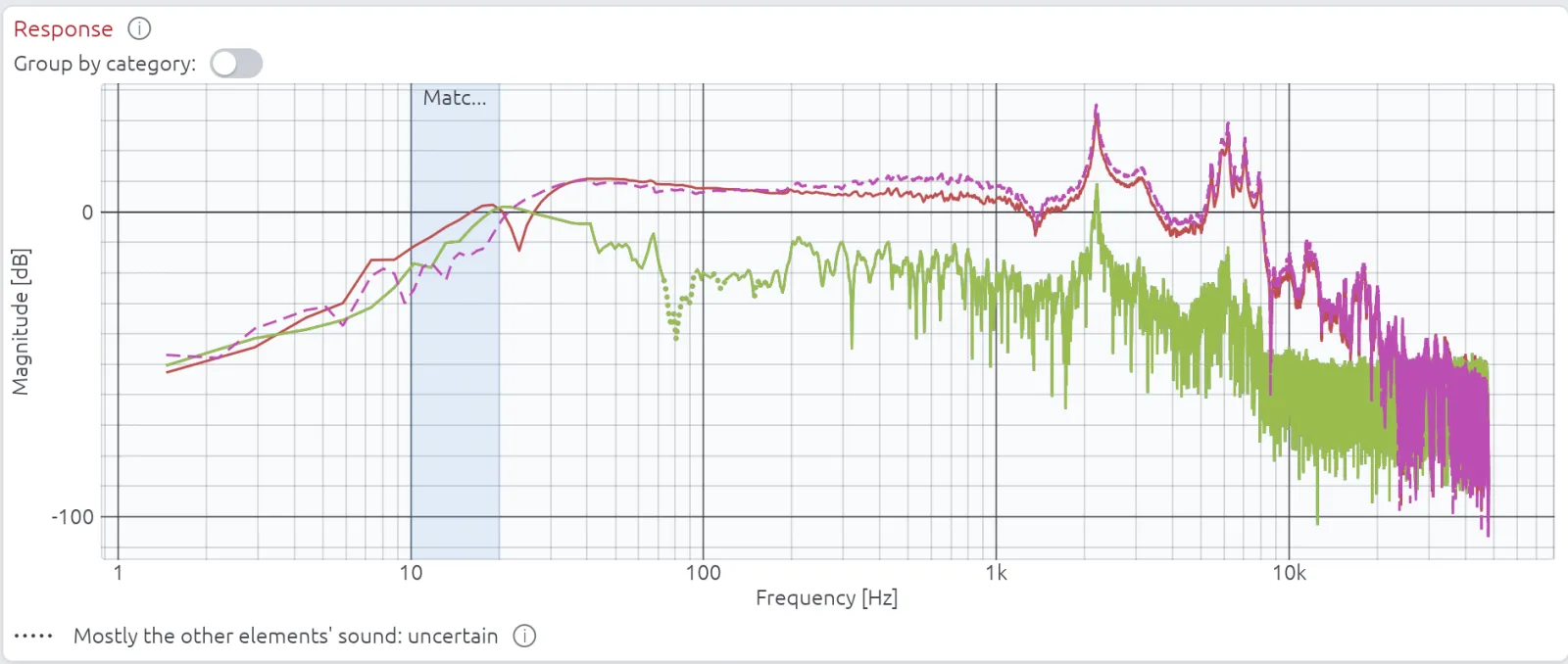
There is nothing to switch on. LinFIR separates the captures whenever two elements or more are placed on the enclosure with their Sd, plus the width and height of a slot vent, which the wizard already asks for to compute delays and diffraction. An element without them is listed above the Response plot and left as captured. Auto-match, the response plot, the predicted response and the spliced measurements all read the separated captures, and the whole solve takes a few milliseconds. A splice applied with an earlier version keeps its results until it is applied again.
8. Next: groups of openings
The same solve is the base for cardioid designs, where the rear wave leaves through several slots on each side, sometimes of different sizes. Each slot can already be captured as a vent with its rectangle. The next step is to let LinFIR handle a row of openings as one group.
9. Conclusion
A near-field microphone hears its neighbours, and in a vented box near the tuning frequency the cone's microphone can hear the port louder than the cone. Solving the captures together removes that cross-talk, with a model of the box that agrees with the boundary elements within a decibel and ten degrees up to 200 Hz on thirteen quite different boxes.
If you find an error, or have near-field captures and a ground-plane measurement of the same speaker to compare, please write to me through the contact page.
How the simulations were made
The boundary element solutions come from Huygens, with the Burton–Miller formulation on a rigid box and triangles of 15 mm around the elements, growing to 50 mm. Each element moves 1 m³/s with a uniform normal velocity over its outline while the others stay still, and the microphones sit 5 mm in front of each element's centre. The thirteen boxes were solved from 20 to 640 Hz in third-octave steps, the vented box of sections 2 and 3 from 12 to 500 Hz in 1/24-octave steps, with its field on a 1 cm grid.
The flows of sections 2 and 3 come from a lumped model at 2.83 V: a driver with Fs 38 Hz, Qes 0.42, Qms 4, Vas 25 L and Sd 154 cm², in 18 L tuned to 45 Hz (Qp 50, QL 10). The separation in the figures uses LinFIR's own coupling matrices, taken from its code.
References
Keele, D. B., Jr., "Low-Frequency Loudspeaker Assessment by Nearfield Sound-Pressure Measurement", Journal of the Audio Engineering Society, 22(3), 154–162, 1974. The near-field method and its scaling.
Struck, C. J. and Temme, S. F., "Simulated Free Field Measurements", Journal of the Audio Engineering Society, 42(6), 467–482, 1994. Near-field and gated far-field measurements spliced together.
Burton, A. J. and Miller, G. F., "The application of integral equation methods to the numerical solution of some exterior boundary-value problems", Proceedings of the Royal Society of London A, 323, 201–210, 1971. The formulation Huygens uses.
Rayleigh, J. W. S., The Theory of Sound, vol. 2, 2nd edition, Macmillan, 1896. The integral for a source in an infinite baffle.
Demion, A., "A Boundary Element Solver on Apple's GPU, Checked Against AKABAK", DEM Audio blog, 2026, /blog/bem-on-the-gpu/. Huygens' solver against exact solutions and AKABAK 3.