
In the previous article I looked at what a near-field microphone hears of its neighbours, and I left Keele's factor itself as it was. This article is about that factor.
The near-field method has a ceiling. The usual rule is \(ka = 1\), with \(a\) the radius of the piston and \(k = 2\pi f/c\), which gives about 840 Hz for a 6.5-inch woofer (a piston radius of 65 mm) and 350 Hz for a 15-inch one (155 mm). Indoors, the gated far-field measurement that takes over above it is only clean from 200 to 400 Hz upwards, depending on the room. For a large woofer in a small room the two bands barely meet, and sometimes they do not meet at all.
I wanted to know how hard that ceiling is. I solved rigid cones in closed boxes with the boundary element solver of Huygens, my loudspeaker design software, and compared the far field predicted from the near-field pressure with the one the solver gives. Along the way I also looked at how precisely the microphone has to be placed, and I found an error of level I had not suspected. Then I set the whole splice against the measurements of a real subwoofer, and found a second one.
1. Where ka = 1 comes from
For a rigid piston of radius \(a\) in an infinite baffle that moves a volume velocity \(U\), the pressure on its axis at a distance \(d\) is known exactly:
$$\begin{gathered} p = \frac{\rho c\,U}{\pi a^2}\left(e^{-ikd} - e^{-ik\sqrt{d^2+a^2}}\right), \\ |p| = \frac{2\rho c\,U}{\pi a^2}\,|\sin x|, \qquad x = \frac{k}{2}\left(\sqrt{d^2+a^2}-d\right) . \end{gathered}$$
At low frequency \(\sin x \approx x\), and this becomes the factor of the previous article,
$$|p| \approx \omega\rho\,U\,\frac{\sqrt{d^2+a^2}-d}{\pi a^2} .$$
The near-field pressure then follows \(\omega U\), as the far field does, and the two differ by a constant. Keele's method takes that constant. With the microphone close to the piston, replacing \(\sin x\) by \(x\) costs 0.36 dB at \(ka = 1\) and 1.5 dB at \(ka = 2\).
Nothing forces that step. Dividing the capture by the exact expression gives the volume velocity for as long as the cone moves as a rigid piston. But a cone is not flat, and it sits in a box whose edges are a few centimetres from the microphone. What is the exact formula worth on such a shape?
2. Two cones in their boxes
I took a 17 cm woofer in a box of 25 × 40 × 30 cm, and a 30 cm one in 40 × 60 × 35 cm. Their piston radii are 65 mm and 130 mm. A driver is named after its frame, and its piston is the disk of the same area as its cone and part of its surround, its Sd. The 12-inch Dayton Audio RSS315 of section 5 has 506.7 cm², a radius of 127 mm. Each is a rigid straight cone with a domed dust cap whose top lies 20 mm and 45 mm behind the cone's edge. I solved them from \(ka = 0.25\) to 4, which is 210 Hz to 3.4 kHz for the small one and half that for the large one, and read the pressure 5 mm from the top of the cap.
That pressure is turned into a volume velocity in three ways: with Keele's constant, with the exact formula above, and with a flat piston solved by boundary elements on the same box, read at the same 5 mm. Each estimate is then radiated by a flat piston of the same area on the box, which is what a splice's model does, and compared with the cone's true far field on the axis.
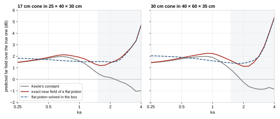
All three curves sit 1.5 to 2 dB above zero at low frequency. I come back to that offset in section 4. Here only the shape matters, since a splice matches the level to the far-field measurement anyway.
Keele's constant holds its level within half a decibel up to \(ka = 1\), then falls away. At \(ka = 2\) it is 1.3 dB under its low-frequency value for the small cone and 1.7 dB for the large one. With the exact near field the curve stays within a band about 1 dB wide up to \(ka = 2.5\).
Most of what moves below \(ka = 2\) is the box. The edges of the baffle send a little sound back to the microphone, which a formula written for an infinite baffle ignores. With the flat piston solved on the box in place of the formula (dashed), the band narrows to 0.3 dB for the small cone and 0.6 dB for the large one.
Above \(ka = 2.5\) all three leave together. The cone's own cavity then shapes what it radiates, and no pressure read on its axis can tell. It shows off the axis first: from 30° to the back of the box, a flat piston's directivity is the cone's within 0.15 dB up to \(ka = 2\), and 2 to 4 dB away from it at 60° and 90° at \(ka = 3.2\).
For a rigid cone, then, the near field holds up to \(ka = 2\) at least. A real cone is not rigid, and the woofer of section 6 followed its capture only up to \(ka = 1.5\), where LinFIR now stops. For a 15-inch woofer that is 525 Hz in place of 350.
3. How precisely the microphone has to be placed
I expected the placement to become critical above \(ka = 1\). It does not.
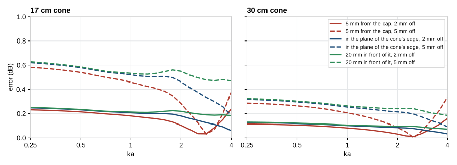
Along the axis, a millimetre costs 0.12 dB for the 17 cm cone and 0.06 dB for the 30 cm one, about \(8.7/a\) dB with \(a\) in millimetres. It is the same 5 mm from the cap, in the plane of the cone's edge and 20 mm in front of it, and it hardly changes with frequency up to \(ka = 3\). Across the axis the pressure is almost flat, and 10 mm cost less than 0.15 dB up to \(ka = 2\).
So a woofer's microphone placed within 2 mm is placed well enough, and there is no need to go as close to the cap as possible. A small port is more demanding. By the same rule a 5 cm port would cost 0.35 dB per millimetre, though I did not simulate one here.
4. A cone is not a flat piston
Back to the offset. For the same volume velocity, the microphone 5 mm from the cap of the 17 cm cone reads 1.9 dB more than it would 5 mm from a flat piston. The air at the bottom of a cone is held between its walls, and it takes more pressure to move it out.
Keele's factor is a flat piston's, so it reads the cone's volume velocity 1.9 dB too high. A driver alone in a closed box never shows it, because the level is matched to the far-field measurement afterwards. It shows as soon as the cone is weighed against a flat radiator. In a vented box the port's capture has no such excess, and the cone counts 1.9 dB too loud against it. An absolute check against an SPL calibration is off by the same amount.
To see what sets that excess I solved 19 more cones beside the flat piston of their area: cones from 0.15 to 0.8 radius deep, a cap from 0.2 to 0.5 radius across, flat, domed or hollow, a tall bullet in place of the cap, a curved cone, and some of them again at twice the size.
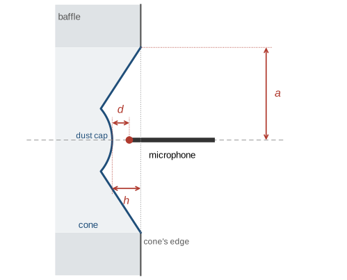
One length says nearly all of it, which is the depth \(h\) of the top of the cap behind the cone's edge.
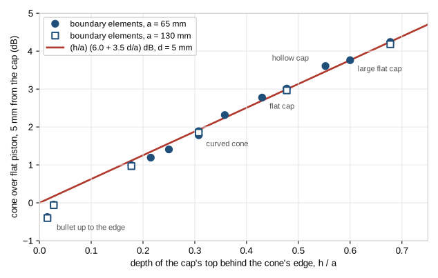
The two sizes fall on the same points, so only ratios count, and a straight line through them gives
$$\Delta L = \frac{h}{a}\left(6.0 + 3.5\,\frac{d}{a}\right)\ \text{dB} .$$
A usual cone, with \(h = 0.3\,a\), reads 1.9 dB high. A deep one at \(0.68\,a\) reads 4.2 dB high. Over all the cones and microphone distances up to half a radius, the line is 0.18 dB off on average. The worst case is the bullet that comes up to the cone's edge. It reads 0.4 dB under a flat piston where the line says 0.1 dB over.
This also answers a practical question, which is what to measure on a driver with a tall cap. The depth is taken from the cone's edge to the point the microphone's distance is measured from. With a bullet that reaches the edge it is zero, and so is the correction. It does not have to be measured finely either: 3 mm change the level of a 17 cm cone by 0.3 dB, and half that for a 30 cm one.
Why a constant is enough
The excess is not the same at every frequency. It grows towards \(ka = 1.5\), where the cone's cavity starts to act as a short horn.

But the far field on the axis grows with it. Over the flat piston, the usual cone gains 1.5 dB at \(ka = 1\) and 2.4 dB at \(ka = 2\). What the microphone reads in excess up there is output the listener gets too. The difference between the two stays within 0.4 dB of its low-frequency value up to \(ka = 2\) for the usual cone, and within 0.9 dB for the deep one. The correction to apply is therefore the low-frequency excess, the same at every frequency.
5. The box between the cone and the microphone
A near-field capture, scaled as above, gives the volume velocity of one element. A splice needs more than that. It has to say what the far-field microphone receives from that element on its box, with the gain of the baffle and the ripple of its edges, and with what goes round to the sides and the back. All of it is one transfer function for each element and each direction, the sound of the element on its box over that of a point source of the same flow in free space.
LinFIR took it from an edge diffraction model, the distributed edge dipole model of Urban and his colleagues [7], in which each edge of the face an element sits on radiates again. The boundary element solver that solved the cones can solve the box itself, with every element a flat piston flush with its face. I put it into LinFIR and compared the two on a project of mine.
Its subwoofer has a 12-inch Dayton Audio RSS315 on the front of a box of 38 × 50 × 52 cm, and a 12-inch passive radiator on each side. The dust cap of the woofer comes up to the cone's edge, so by section 4 its capture needs no correction. Its midwoofer, a coaxial of 78 cm², has a box of 17 × 26 × 17 cm to itself. Each was measured on a turntable every 10°, with the microphone at 79 cm and a time window of 12 ms (11 ms for the midwoofer), which holds from 366 Hz upwards (274 Hz). The near-field captures were taken 5 mm from the woofer and the passive radiators, and 10 mm from the midwoofer.
Seen from the woofer
The two models agreed with each other, and both missed the measurement by more than they differed. The reason was in where the microphone stood. It was on the speaker's reference axis, the one the microphone is aimed along, which passes 72 cm above the woofer.
LinFIR read each element's transfer function far away, in the direction of the microphone as seen from the reference point. For the midwoofer nothing is wrong with that, since it is at the reference point. Seen from there the microphone is straight ahead, so the woofer was read on its own axis. Seen from the woofer, the microphone is 42° up.
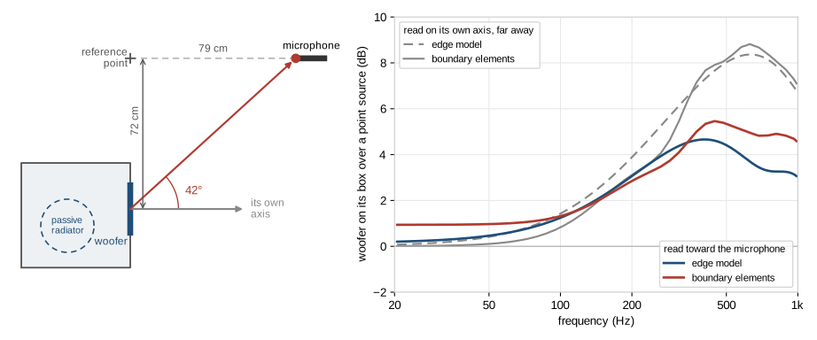
On its axis the woofer gets 7 to 8.5 dB from its baffle between 366 and 645 Hz, and the two models say so within 0.4 dB. Toward the microphone it gets 3.5 to 5.5 dB. A splice sets the level of the prediction where it overlaps the far-field measurement, here from 366 to 645 Hz. With 3.5 dB too much baffle on average in that band, the level came out 3.5 dB too low, and the whole bass with it. This error is older than this study, and it touched every element far from the reference point.
Each element is now read as the microphone saw it. The boundary element solution gives the field anywhere outside the box, so it is read at the microphone's own place. The edge model gives a far field, and is read in the microphone's direction from the element.
At low frequency the boundary elements sit 0.9 dB above zero. Close to the box, compared with its size, the woofer radiates into half the space, and far away into all of it, at any frequency low enough. At 1.07 m from this box its sound is still 0.9 dB above that of a point source at the woofer, as if it came from a point about 15 cm in front of it, its acoustic centre [8]. Read 30 m away, the boundary elements give 0 dB.
Element by element
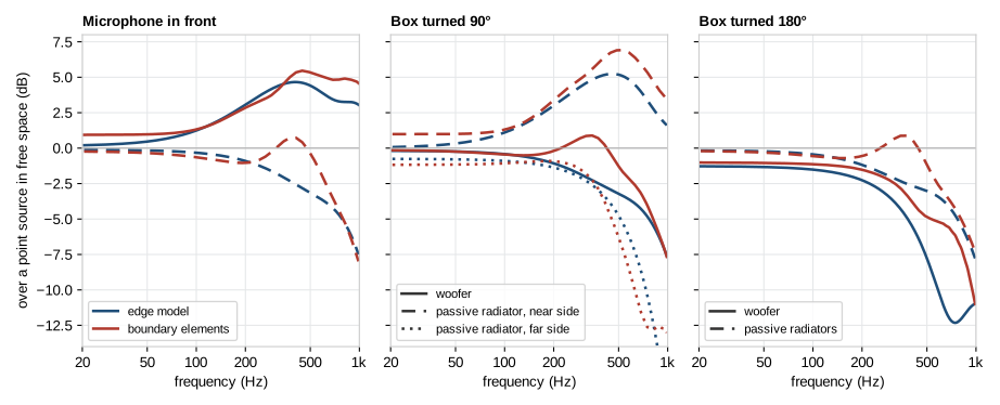
With the microphone in front, the two models give the woofer the same transfer function within 0.6 dB up to 400 Hz. Above, the boundary elements keep 1.2 to 1.6 dB more.
They part for an element the microphone sees from the side. That is the case of the passive radiators with the microphone in front, and of the woofer once the box is turned 90°. Near 400 Hz the boundary elements show a bump of half a decibel where the edge model has already lost 2.5 dB. The edge model knows the edges of the face an element is on. The box is 52 cm deep, and the sound that goes round it meets its other edges too.
Behind the box the woofer is 10.5 dB down at 600 Hz by the edge model, and 5.3 dB by the boundary elements.
6. Against the measurements
I have no anechoic measurement of this speaker to judge the two models by. The gated one stops at 366 Hz. Below that it still holds the direct sound, blurred by its 12 ms window, and the prediction can be passed through the same window. The two are then compared like with like, down to about 100 Hz. Nothing narrower than 80 Hz shows through such a window, which leaves the level and the slope of the response.
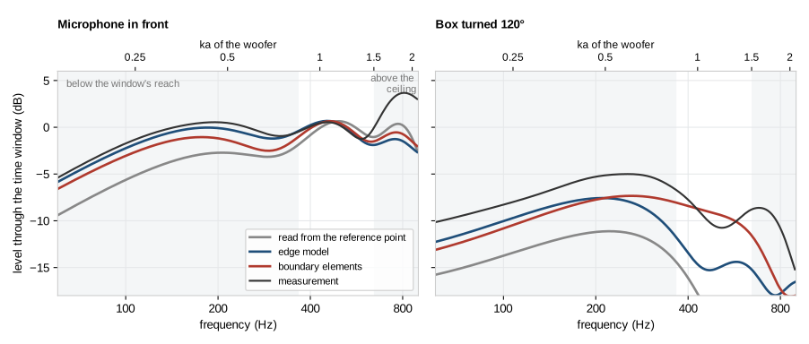
With the microphone in front, the edge model runs 0.3 to 0.7 dB under the measurement from 60 to 300 Hz, and the boundary elements 1.2 to 2 dB under. The former reading was 2.3 to 4 dB under. With the box turned 120° both run 1.8 to 3 dB under the measurement up to 200 Hz. From 300 to 600 Hz the boundary elements stay within 2.2 dB of it, and the edge model falls 3.8 to 5.7 dB under.
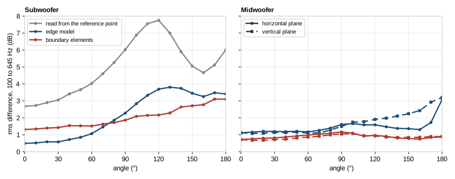
Over the 37 angles of the subwoofer's horizontal plane, from 100 Hz to its ceiling at 645 Hz, the prediction was 5.3 dB from the measurement with the former reading. It is 2.6 dB with the edge model and 2.1 dB with the boundary elements. Within 60° of the axis the edge model is the closer of the two, 0.7 dB against 1.5 dB. From 90° to the back it is 3.4 dB against 2.5 dB. The subwoofer's vertical plane was not measured. It is a copy of the horizontal one, as LinFIR allows for a subwoofer, and was left out.
The midwoofer is at its reference point, so the reading changes nothing for it and what is left is the two models. Over its 73 angles in both planes the prediction is 1.7 dB from the measurement with the edge model and 0.9 dB with the boundary elements. Straight behind its box the edge model is 3.1 dB off, the boundary elements 0.9 dB.
For the subwoofer, most of the gain came from where each element is read from. The boundary elements add to it at the sides and behind, and for the small box at every angle. In front of the subwoofer they do worse than the edge model, because they put its bass 1.2 to 2 dB under the measurement. Both are matched in level between 366 and 645 Hz, so from that band down to the bass the measurement falls less than the boundary elements predict. I cannot tell from these data whether the woofer's capture already reads a little high in that band, as a cone that starts to break up would, or whether the solved baffle gives a little too much. Behind the box both models run 3 to 4 dB under the measurement in the bass.
I think most of what is left comes from how this speaker was measured. The subwoofer holds 60 litres and is heavy, and I did not raise it on the turntable as high as I would have liked. Half a decibel of precision did not seem worth a subwoofer on the floor. The floor was then closer than I wanted, and the time window keeps its reflection, which the prediction, solved in free space, does not have. The midwoofer's near-field capture was taken 10 mm from the plane of the bottom of its cone, in front of the small waveguide that holds its tweeter. None of the cones of section 4 looks like that. I will take other measurements when I have the time.
The spliced responses
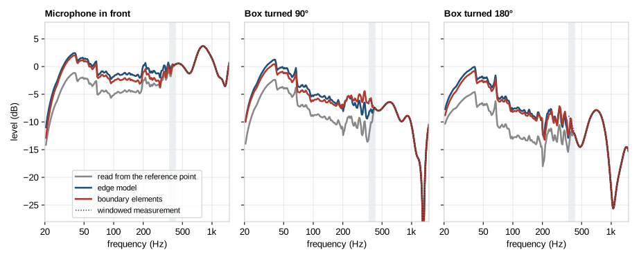
In the splice, the new reading lifts the subwoofer's bass by 3.3 dB on the axis with the edge model and by 2.6 dB with the boundary elements, and by more than 4 dB behind the box. The steps near 42, 67 and 197 Hz are in the near-field captures themselves.
Where this woofer stops
This woofer is also the first real driver I can set against section 2, and the upper axis of the windowed responses above gives its \(ka\). Up to \(ka = 1.45\), which is 620 Hz, the prediction sits within 0.7 dB of the measurement on average, on the axis and 30° either side. Above, the measurement climbs away from it. The prediction is 1.2 to 1.7 dB under between \(ka = 1.45\) and 1.6, and 4 to 5 dB under between 1.6 and 2. The two models miss it alike, and the passive radiators change the sum by less than a decibel there, so it is the woofer's own capture that no longer says what the woofer radiates. Matching the level up to \(ka = 2\) instead, as LinFIR did before, moves both sides of that step by 0.7 dB and leaves the step.
One woofer is thin evidence, and this one is seen from 42° above its axis. The rigid cones of section 2 gave 2.5, and this woofer stopped near 1.5. LinFIR now stops there too.
7. What this does not cover
The cones of sections 2 to 4 are rigid. A real one stops moving as one piece somewhere, and from there its pressure on the axis says little about its far field. The one real woofer of section 6 did so near \(ka = 1.5\), well below the 2.5 the rigid cones allowed, and LinFIR stops there. Another woofer may hold longer or stop sooner.
Deep cones, curved cones and large caps drift a little more with frequency than the two of section 2, up to 1 dB at \(ka = 2\). The transition band of a splice, where the far-field measurement takes over progressively, spreads that out.
I did not simulate a phase plug that stands still, a surround with its roll, or a port, whose air does not move at its mouth as a piston does.
The measurements of sections 5 and 6 are gated measurements in a room, compared with the prediction through their own window. They test the box's part of the splice and the level it sets, down to about 100 Hz. They are not an anechoic reference, and each box is solved alone in free space, without what stood near it. I still have no ground-plane measurement of a driver between \(ka = 1\) and \(ka = 2\).
8. In LinFIR
From version 1.5.6, the splicing wizard divides each near-field capture by the exact near field of its outline, a disk for a cone, a passive radiator or a round port and a rectangle for a slot vent, and takes the near field up to \(ka = 1.5\). The valid blend range of the wizard is that much wider. The line under each element shows its new ceiling, and the transition band still stays under 1000 Hz. Below \(ka = 1\) a capture changes by 0.36 dB at most, and a splice applied with an earlier version keeps its results until it is applied again.
Drivers and passive radiators get a new field in the first step, Cap depth. It takes the depth \(h\) and brings the capture down by the excess above. Left at 0, everything is as before. The wizard's level-matching step could already hide the error for a vent, by fitting its curve to the cone's below the tuning frequency, but that fit does not hold for a passive radiator. With the depth, the level comes from the geometry.
The enclosure is solved by boundary elements, once and in the background, with all its elements together. Up to 1000 Hz, every angle of the polar measurements is then read from that one solve. It takes less than a second on a Mac, where it runs on the GPU. On Windows and Linux it runs on the CPU, which took 7 s for a small box and 30 s for a floorstander with three elements on the same Mac. A setting brings back the edge model.
Both models read each element as the microphone saw it. For a driver at the reference point nothing changes. For a subwoofer measured on another driver's axis the bass of the splice moves by a few decibels, as above. A splice applied with an earlier version keeps its reading and its results until it is applied again from the wizard, whose last step says when the two differ.
9. Conclusion
The ceiling at \(ka = 1\) belongs to Keele's constant more than to the near field. With the exact near field of a piston, the capture of a rigid cone stands for its far field up to \(ka = 2\) within about half a decibel, with a microphone placed to a couple of millimetres. And a cone reads louder up close than the flat piston the method assumes, by an amount the depth of its dust cap gives within a few tenths of a decibel.
Set against the measurements of a real subwoofer, the splice had a larger error than any of these. Its elements were read in the direction of the reference point, 42° away from where the microphone saw the woofer, and its bass came out 3.5 dB too low. Read as the microphone saw them, the prediction is 2.6 dB from the measurement over the subwoofer's 37 angles with the edge model and 2.1 dB with boundary elements, which also bring a midwoofer from 1.7 to 0.9 dB over its 73 angles. Most of what is left comes, I think, from how I measured that speaker. The subwoofer's cone followed its capture up to \(ka = 1.5\), and LinFIR takes the near field that far.
If you find an error, or have near-field captures and a ground-plane measurement of the same driver to compare, please write to me through the contact page.
How the simulations were made
The boundary element solutions come from Huygens, with the Burton–Miller formulation on a rigid box. Each frequency is solved on its own mesh, with triangles of 6 mm on the 17 cm cone and 12 mm on the 30 cm one, growing to 40 mm away from it. On a mesh one and a half times finer, the far field moves by less than 0.05 dB and the near pressure by 0.01 dB.
The cone moves along its axis as one rigid body, 1 m³/s, with its edge in the plane of the baffle and no surround. The two cones of sections 2 and 3 were solved at 25 frequencies, a sixth of an octave apart. The nineteen cones of section 4 and their flat pistons were solved at seven frequencies from \(ka = 0.125\) to 2.5 and read from 3 to 60 mm from their cap. The line is fitted at \(ka = 0.125\) on the 145 readings taken within half a radius of the cap.
How the comparison with the measurements was made
In LinFIR the same solver takes the box alone, its elements flat pistons flush with their faces, from 20 Hz to 1250 Hz at eight frequencies an octave. The subwoofer's box has 1550 triangles and the midwoofer's 432. Their transfer functions are used up to 1000 Hz.
The comparison goes through LinFIR's own splice. The level of the prediction is matched to the windowed measurement on the axis over the band where the two overlap, 366 to 645 Hz for the subwoofer and 274 to 1000 Hz for the midwoofer, and its time offset on the transition band, 366 to 430 Hz and 535 to 671 Hz, as the wizard's two buttons do. Each model gets its own level and offset. A difference is the rms value of the difference in decibels on 48 points an octave from 100 to 645 Hz, then over the angles.
References
Keele, D. B., Jr., "Low-Frequency Loudspeaker Assessment by Nearfield Sound-Pressure Measurement", Journal of the Audio Engineering Society, 22(3), 154–162, 1974. The near-field method and its scaling.
Struck, C. J. and Temme, S. F., "Simulated Free Field Measurements", Journal of the Audio Engineering Society, 42(6), 467–482, 1994. Near-field and gated far-field measurements spliced together.
Kinsler, L. E., Frey, A. R., Coppens, A. B. and Sanders, J. V., Fundamentals of Acoustics, 4th edition, Wiley, 2000. The pressure on the axis of a baffled piston.
Burton, A. J. and Miller, G. F., "The application of integral equation methods to the numerical solution of some exterior boundary-value problems", Proceedings of the Royal Society of London A, 323, 201–210, 1971. The formulation Huygens uses.
Demion, A., "What a Near-Field Microphone Really Hears", DEM Audio blog, 2026, /blog/near-field-cross-talk/. The captures of a box's elements solved together.
Demion, A., "A Boundary Element Solver on Apple's GPU, Checked Against AKABAK", DEM Audio blog, 2026, /blog/bem-on-the-gpu/. Huygens' solver against exact solutions and AKABAK 3.
Urban, M., Heil, C., Pignon, C., Combet, C. and Bauman, P., "The Distributed Edge Dipole (DED) Model for Cabinet Diffraction Effects", Journal of the Audio Engineering Society, 52(10), 1043–1059, 2004. The edge model.
Vanderkooy, J., "The Acoustic Center: A New Concept for Loudspeakers at Low Frequencies", 121st Convention of the Audio Engineering Society, paper 6912, 2006. Where a box's low-frequency sound comes from.