For some time now I have been working on a new tool, called Huygens, for loudspeaker design. I will say more about it when it is ready. Underneath it there is a boundary element solver (BEM), the method that computes how a cabinet, a waveguide or a horn radiates sound. This article is about that solver, and about one question: can its curves be trusted?
A simulation that cannot be checked is worth very little. So before designing anything with it, I compared it with two kinds of reference:
- exact solutions, problems simple enough that the right answer is known with pencil and paper;
- AKABAK 3, the software most of the trade uses for this kind of computation.
The short version:
- On a waveguide, Huygens and AKABAK draw the same curves: 0.007 dB apart in the median, 0.30 dB at most, at 16 kHz far off the axis.
- On a closed body, a sphere whose exact solution is known, Huygens stays within 0.13 dB at every frequency. With its default settings, AKABAK strays by up to 2.4 dB at the frequencies where the classical method is known to break down.
- AKABAK's polars are computed in the far field, then scaled to the distance you ask for. For a near-field design, that matters.
- On a Mac mini M4 Pro, Huygens solves a complete waveguide, 40 frequencies from 1 to 20 kHz, in 1.2 seconds.
A note on intent. AKABAK is a serious, well-established piece of software, and this is not a takedown. It is used here because it is the reference: if a new solver disagrees with AKABAK, the burden is on the new solver. Where the two differ, I show the exact solution that decides between them, and how the comparison was set up, so that anyone with AKABAK can redo it.
1. The method, briefly
The boundary element method solves the wave equation in the air around an object by meshing only its surface. The air around it, out to infinity, is taken into account exactly by an elementary solution of the wave equation (the Green's function): no volume of air to mesh, no artificial boundary to make absorbing. Once the surface pressure is known, the pressure anywhere in space (polars, directivity maps) follows from an integral over the surface.
Huygens uses the textbook ingredients, done carefully:
- a Galerkin formulation, where the equations hold on average over each triangle rather than at a few points: more expensive integrals, but more accurate and more forgiving of irregular meshes;
- the Burton–Miller formulation for closed bodies, which removes the "irregular frequencies" discussed in section 4;
- dedicated quadratures for the singular integrals, where two elements touch or nearly touch, as in the tight corner of a waveguide's mouth;
- the infinite baffle through the half-space Green's function, and symmetry: a symmetric waveguide is solved on its quarter, four times fewer unknowns.
None of this is new. What is less common is where it runs.
2. Why it is fast: Apple Silicon's GPU and its shared memory
Most of the time in a BEM computation goes into building the system: for every pair of triangles, an integral of the Green's function. There are millions of these pairs, all independent of each other, which is exactly the kind of work a GPU is built for.
On Apple Silicon, Huygens builds the system on the GPU, through Apple's Metal framework, in single precision. The system is then solved by an iterative method on the CPU. The detail that makes the difference is that the CPU and the GPU share the same memory. On a PC with a graphics card, a matrix built by the GPU has to be copied across the bus before the CPU can use it. On an Apple Silicon Mac, the CPU reads it where the GPU wrote it, with no copy. So the two work in a pipeline: while the CPU solves one frequency, the GPU is already building the next one.
Accuracy is not sacrificed for speed. Every change to the code is checked, in continuous integration, against a double-precision computation on the CPU, and the timings below are measured on the same Mac mini at every change.
3. The reference: a cap vibrating on a sphere
The problem
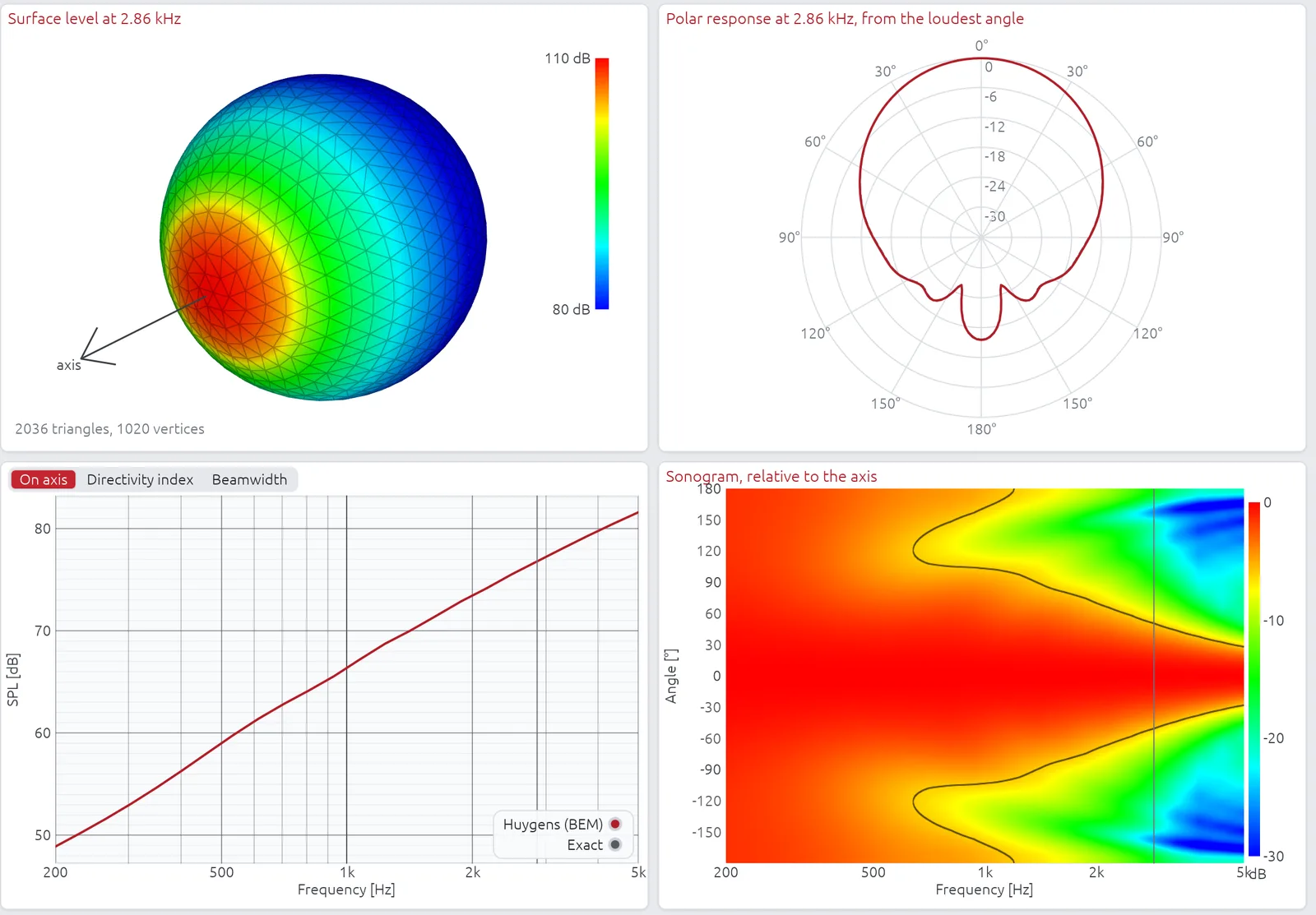
A rigid sphere of radius \(a\) = 100 mm, in free field. A cap of half-angle \(\theta_0\) = 30° around the axis vibrates: each of its points moves along the radius at the same velocity \(u\), and the rest of the sphere stays still. It is often called the "piston on a sphere", and it is the textbook model of a driver in a spherical cabinet.
A word on the name. A real piston, or a dome, translates along the axis as a rigid body; here, every point of the cap moves along its own radius. It is an idealisation of a driver, but one with an exact solution, which makes it the perfect test for a solver: the right answer is known to every digit.
Why an exact solution exists
The cap is convex, and that is not an obstacle but the very condition: the cap is part of the sphere, so the whole boundary is still a sphere, and in spherical coordinates the wave equation separates. A flat piston set into the sphere, or a dome of another radius, would break that, and with it the exact solution.
The velocity on the sphere is expanded in Legendre polynomials. For the cap, the coefficients are simple:
$$ v(\theta) = \sum_{n \ge 0} V_n P_n(\cos\theta), $$
$$ V_0 = \frac{u}{2}(1 - \cos\theta_0), \qquad V_n = \frac{u}{2}\left[P_{n-1}(\cos\theta_0) - P_{n+1}(\cos\theta_0)\right]. $$
Each Legendre term radiates on its own, as an outgoing spherical wave. Outside the sphere, with the time dependence \(e^{-i\omega t}\) and the spherical Hankel functions \(h_n = j_n + i y_n\),
$$ p(r, \theta) = \sum_{n \ge 0} A_n h_n(kr) P_n(\cos\theta), \qquad A_n = \frac{i \rho c V_n}{h_n'(ka)}, $$
where \(A_n\) follows from the boundary condition on the sphere, \(\partial p / \partial r = i\omega\rho v\) at \(r = a\). Far away, \(h_n(kr) \to (-i)^{n+1} e^{ikr} / (kr)\), and the pressure becomes a directivity divided by the distance:
$$ p(r, \theta) \to \frac{e^{ikr}}{kr} \sum_{n \ge 0} (-i)^{n+1} A_n P_n(\cos\theta). $$
Keep this last formula in mind: it is what AKABAK reports (section 5).
How many terms?
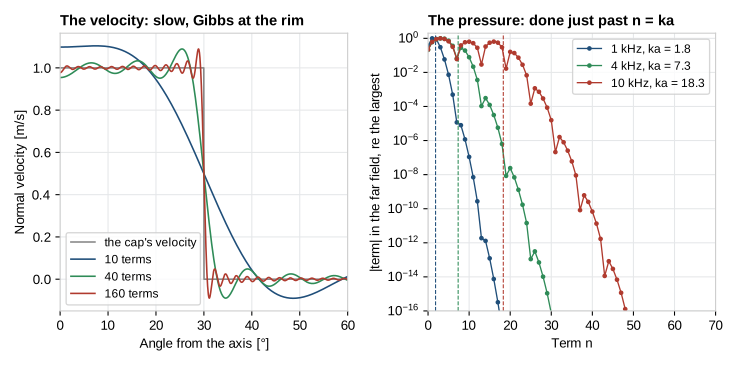
The velocity series converges badly: the velocity jumps at the rim, and the series overshoots there however many terms are kept (left). The pressure series does not have this problem (right): the terms stop counting once \(n\) passes \(ka\), and \(ka + 40\) of them give the result to machine precision. The reason is physical. Term \(n\) is a pattern of \(n\) lobes around the sphere, and lobes finer than the wavelength do not radiate: they stay attached to the surface.
What the solution shows
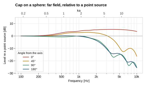
Relative to a point source of the same volume velocity, the curves tell the story of every closed cabinet.
- Below about 300 Hz (\(ka\) < 0.5), the sphere is small compared with the wavelength and the cap radiates like a point source, with the same level in every direction.
- Then the sphere becomes a baffle. On the axis the level rises, +3.9 dB at 1 kHz and about +5 dB from 2 to 6 kHz: the baffle step, which on a sphere is a smooth transition. At 90° and behind, the level falls: the sphere casts a shadow, −17 dB at 90° and −14 dB behind at 4 kHz.
- Above \(ka \approx 5\) (2.7 kHz), the cap itself, 104 mm across, starts to beam: the level at 45° drops by more than 10 dB past 5 kHz.
Radial or rigid?
A cap translating along the axis as a rigid body, like a real dome, has a normal velocity \(u\cos\theta\) on the cap instead of \(u\). Its Legendre coefficients are different, but the solution is just as exact, so the idealisation can be measured.
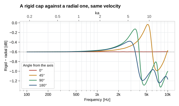
On the axis, the two differ by −0.6 dB at every frequency. Over a 30° cap, \(\cos\theta\) stays between 0.87 and 1, and what remains is the ratio of their volume velocities, \((1 + \cos\theta_0)/2\). Off the axis, above 3 kHz, the difference reaches 1.3 dB. So the "piston on a sphere" is close to a real dome, but not identical. For testing a solver this does not matter at all: Huygens, the exact solution and AKABAK are all given the same radial velocity, and the agreement below shows that AKABAK applied it too.
4. Huygens and AKABAK on the sphere
The test case
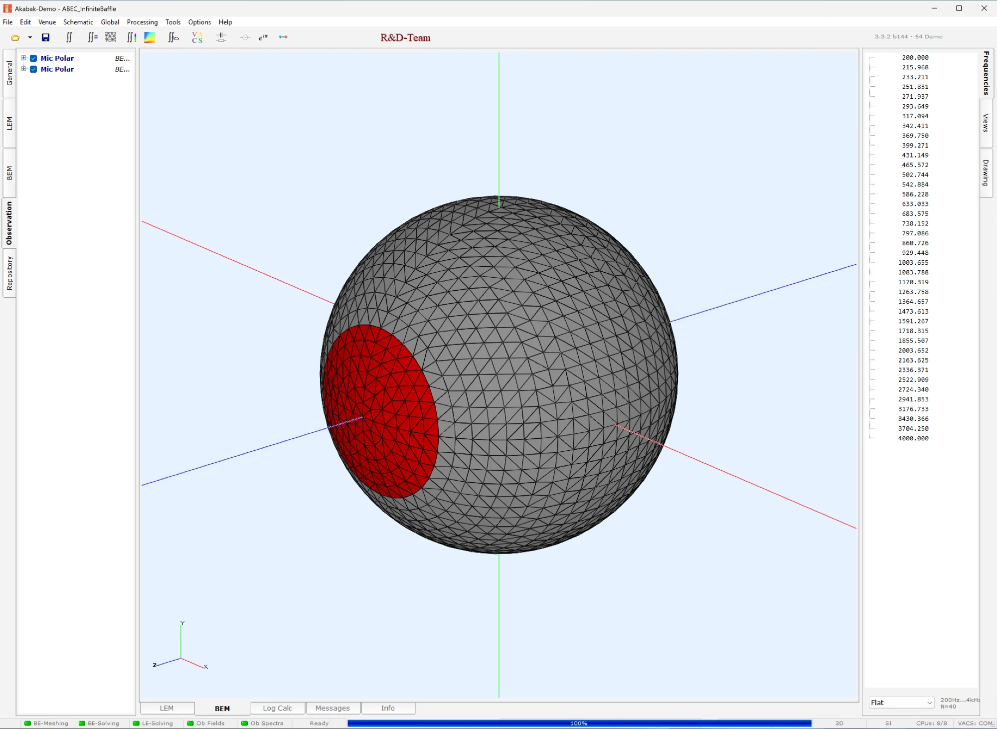
The cap above, meshed with 2736 triangles (10 mm edges). AKABAK solved the very same mesh, a quarter sphere mirrored twice. Forty frequencies from 200 Hz to 4 kHz, polars from 0 to 180° in steps of 5°.
What irregular frequencies are
The classical boundary integral equation has a known flaw. For a closed body, at certain frequencies, its solution is no longer unique. These are the resonance frequencies of the inside of the body, as if it were filled with air and its walls were pressure-release. There is no air inside a BEM model, yet the equation still "hears" these resonances, and the computed exterior field goes wrong.
For a sphere of radius \(a\), they fall where a spherical Bessel function vanishes, \(j_n(ka) = 0\): the same functions as in the exact solution, here describing the air that is not inside the sphere. In our band that means \(ka = \pi\) (1715 Hz), 4.49 (2453 Hz), 5.76 (3146 Hz), \(2\pi\) (3430 Hz) and 6.99 (3815 Hz).
This is not a sphere curiosity. Every closed cabinet has them. For a rectangular box of inner dimensions \(L_x \times L_y \times L_z\), the first one is at
$$ f_1 = \frac{c}{2}\sqrt{\frac{1}{L_x^2} + \frac{1}{L_y^2} + \frac{1}{L_z^2}} $$
that is, about 1.1 kHz for a 20 × 30 × 40 cm box, right in the crossover region of a two-way speaker. More follow, closer and closer together, as the frequency rises.
The result
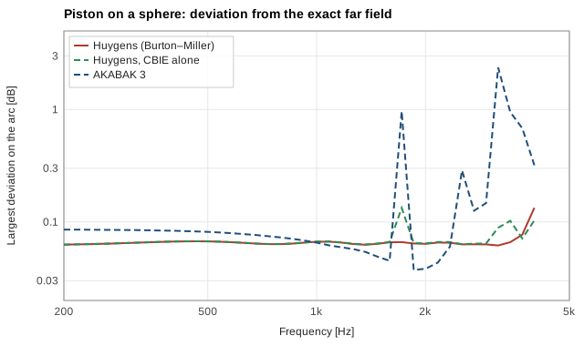
- Huygens with Burton–Miller (its default): 0.13 dB at most, 0.065 dB in the median, without a single spike.
- Huygens with the classical formulation (CBIE), without Burton–Miller: small bumps at the irregular frequencies, still 0.13 dB at most. In my runs, the Galerkin formulation is hardly sensitive to them.
- AKABAK, with its default settings: as accurate as Huygens between these frequencies, but spikes of 0.97 dB at 1718 Hz, 0.29 dB at 2523 Hz, 2.36 dB at 3177 Hz, 0.95 dB at 3430 Hz and 0.68 dB at 3704 Hz, the computed frequencies nearest the irregular ones, and still 0.32 dB at 4 kHz as the next one approaches (4217 Hz).
So even with the same classical formulation, without the Burton–Miller remedy, Huygens stays an order of magnitude closer to the exact solution at these frequencies. AKABAK may well offer settings that improve this. The point is what you get by default. And a 2.4 dB spike at a single frequency is dangerous precisely because it looks plausible: on a cabinet's response, it easily passes for a real acoustic effect, a diffraction or a resonance, and someone may end up designing a filter to correct it.
Huygens's residual error, for its part, comes from the mesh, not the method: a faceted sphere is not quite a sphere. It shrinks as the square of the edge length, from 0.068 dB with 16.7 mm edges to 0.009 dB with 5.6 mm edges (table in section 7), as expected of a well-integrated second-order method.
5. AKABAK computes its polars in the far field
When I first compared AKABAK's sphere polars, at 2 m, with the exact pressure at 2 m, they disagreed by about half a decibel: the front too low, the back too high. They do match, within 0.05 dB in the median, the exact far field, scaled back to 2 m by the 1/r law. In other words, AKABAK's polar observation at "2 m" is the far-field directivity, normalised to 2 m.
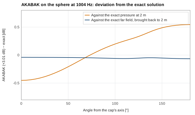
For a source sitting at the centre of the polar arcs, like a waveguide's mouth, the difference is negligible (about 0.01 dB at 2 m). It is not negligible when the source is off-centre, which is the case of almost every driver on a real cabinet. The exact solution shows how much, distance by distance:
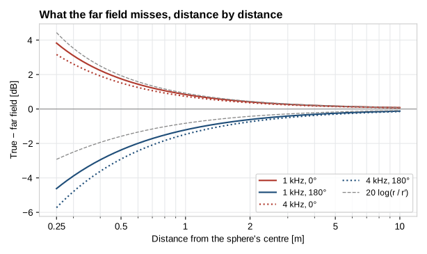
| Distance | In front (0°) | Behind (180°) |
|---|---|---|
| 2 m | +0.4 dB | −0.6 to −0.7 dB |
| 1 m | +0.7 to +0.8 dB | −1.2 to −1.5 dB |
| 50 cm | +1.5 to +1.8 dB | −2.4 to −2.9 dB |
In front, a simple estimate does the job. For a source at a distance \(d\) in front of the rotation centre, the true distance at distance \(r\) and angle \(\theta\) is \(r' = \sqrt{r^2 + d^2 - 2rd\cos\theta}\), and the far field misses
$$ \Delta L = 20 \log_{10} \frac{r}{r'} , $$
+0.45 dB at 2 m for \(d\) = 10 cm. Behind, the error is larger than this estimate: the sound does not cross the sphere, it travels around it, a longer way.
Level is only half of the story. In the far field, all the drivers of a speaker are seen from the same angle. At a real listening distance they are not. A tweeter and a woofer 15 cm apart, listened to at 1 m on the tweeter's axis, differ in path length by 11 mm. That is about 35° of phase at a 3 kHz crossover, which the far field sets to zero. For a far-field PA cabinet, none of this matters. For a near-field studio monitor, a desktop speaker, or anything listened to at a metre or two, the far-field curves describe a listening position nobody occupies.
Huygens computes the pressure at the distance asked for. For the comparisons in this article, it was therefore solved at 2 km and scaled back to 2 m, to compare the same quantity as AKABAK.
6. A waveguide: Huygens against AKABAK
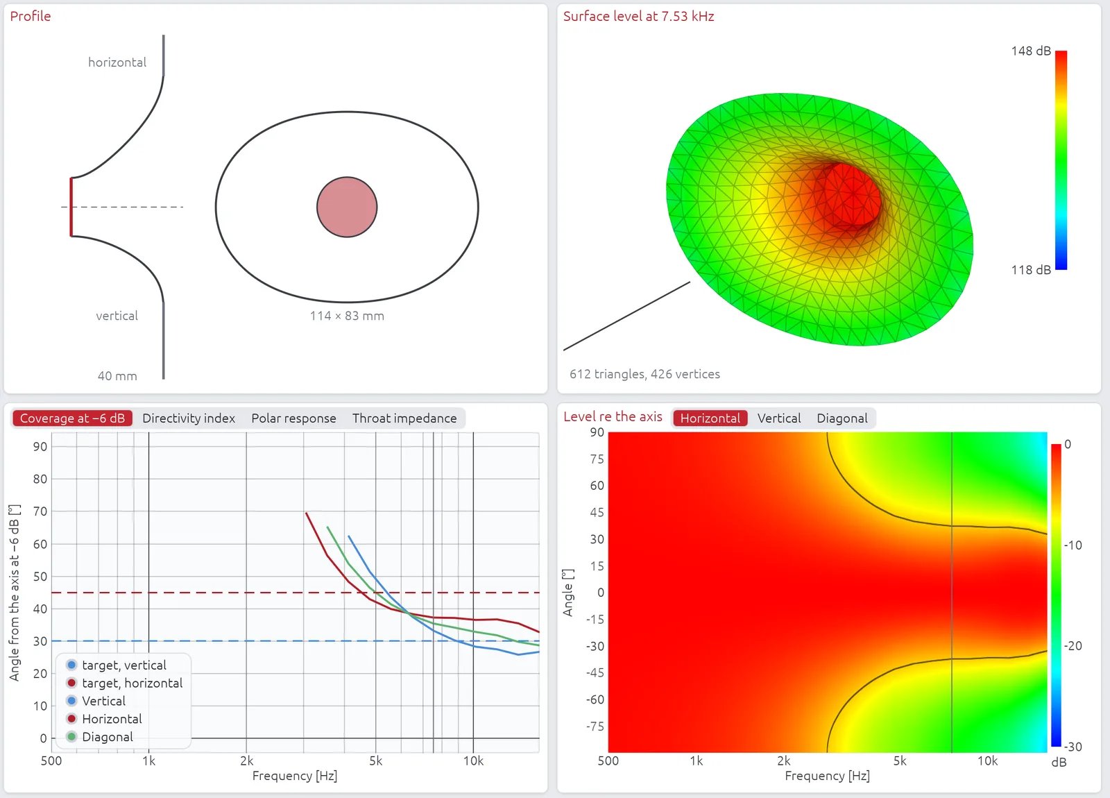
The test case
A small elliptical OS-SE waveguide: a 1-inch throat, 40 mm deep, a 114 × 83 mm mouth, a 45° half-angle horizontally and 30° vertically, in an infinite baffle. It is described once, in an Ath 4.8.2 configuration file. Ath writes the AKABAK project from it, with its mesh (a quarter of 1165 triangles, edges from 0.5 to 5.4 mm). Huygens reads the same file. It can mesh the waveguide itself, or solve Ath's mesh, element for element the one AKABAK solves. The throat is a disc moving at 1 m/s. Forty frequencies from 500 Hz to 16 kHz; horizontal, vertical and diagonal polars from 0 to 90° in steps of 5°: 2280 points in all.
Two conventions had to be aligned. AKABAK reads 1 m/s as a peak velocity and reports RMS levels, so its levels are 3.01 dB below Huygens's at every frequency; that offset is removed everywhere below. And since AKABAK gives far-field polars, Huygens was solved far away and scaled back to 2 m (section 5).
A pitfall for Ath users. AKABAK ignored the baffle offset that Ath writes into the project. On the first run, the baffle sat at the throat, 40 mm behind the mouth, which produced a comb filter: −10 dB on the axis around 1.5 kHz, +6 dB around 2.5 kHz. Shifting the mesh so that the mouth is at z = 0 fixed it. If your AKABAK results for an Ath waveguide look strangely rippled, check this first.
The curves
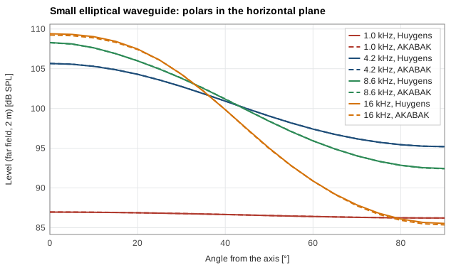
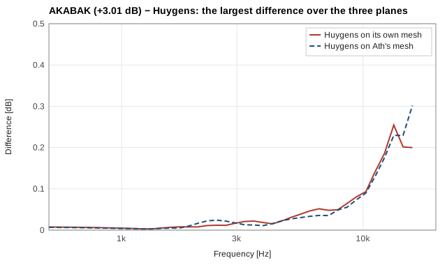
The curves coincide at the scale of the charts, on the axis and off it, up to 16 kHz. On the same elements (Ath's mesh), the difference is 0.007 dB in the median over the 2280 points, 0.01 dB at most up to 2 kHz, and 0.30 dB at most, at 16 kHz far off the axis. With Huygens's own mesh, 0.26 dB at most.
The difference grows with frequency because both solvers approximate the same geometry with elements that become coarse compared with the wavelength: at 16 kHz the wavelength is 21 mm, and Ath's largest elements measure 5.4 mm, four per wavelength. It is largest far off the axis, where the level is low and a small difference in pressure weighs more in decibels.
Which one is closer to the truth?
A waveguide has no exact solution, so the mesh is refined until the result stops moving. The reference is a Huygens solve with 1.5 mm edges (19,008 triangles). Deviation from that reference, over the three planes:
| Frequency | Huygens, Ath's mesh | AKABAK, Ath's mesh | Huygens, its own mesh (2.68 mm) |
|---|---|---|---|
| 1.1 kHz | 0.004 dB | 0.003 dB | 0.004 dB |
| 3.2 kHz | 0.012 dB | 0.016 dB | 0.023 dB |
| 7.2 kHz | 0.057 dB | 0.046 dB | 0.041 dB |
| 12.3 kHz | 0.114 dB | 0.154 dB | 0.080 dB |
| 16 kHz | 0.165 dB | 0.215 dB | 0.101 dB |
On the same elements, the two solvers are as close to the converged solution as each other: a draw, which is what one expects of two correct implementations of the same method. Huygens's own mesh, finer at the mouth, does better above 7 kHz. A fair caveat: the reference is computed by Huygens. Its own uncertainty (the gap between its 2 mm and 1.5 mm meshes) is 0.03 dB up to 9.4 kHz and 0.14 dB at 16 kHz, and only an AKABAK run on a finer mesh would tell what AKABAK converges to.
7. Speed
I could not compare speeds with AKABAK. My copy is the demo version and ran in a virtual machine on a small NAS, so its timings would mean nothing. Beyond that, the two do not run on the same hardware. To my knowledge, AKABAK computes on the CPU and does not use the GPU, while Huygens is built around it.
The times below come from a Mac mini M4 Pro. They are measured automatically at every change to the code.
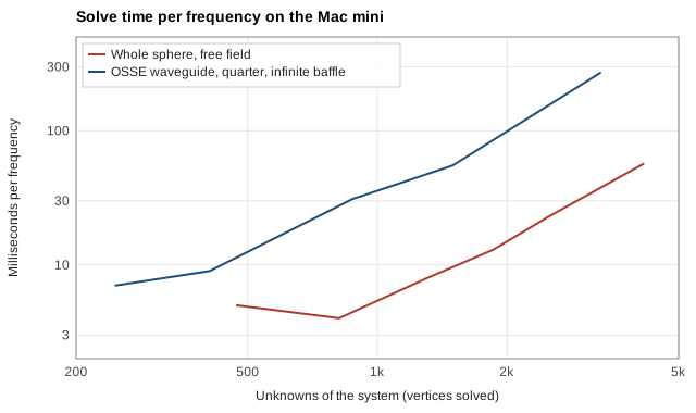
A whole sphere in free field, ten frequencies around 1 kHz, one mesh per row:
| Edges | Triangles | Time per frequency | Deviation from exact |
|---|---|---|---|
| 16.7 mm | 936 | 5 ms | 0.068 dB |
| 10.0 mm | 2610 | 8 ms | 0.026 dB |
| 7.1 mm | 5000 | 23 ms | 0.013 dB |
| 5.6 mm | 8314 | 57 ms | 0.009 dB |
Full sweeps, 40 frequencies, the mesh following the frequency:
| Case | Finest mesh | Total time |
|---|---|---|
| Ath's OSSE example, 1 to 20 kHz | 12,640 triangles | 1.2 s |
| Small elliptical waveguide (section 6), Ath's mesh, 500 Hz to 16 kHz | 4660 triangles | 4.2 s |
| Same, Huygens's mesh | 6216 triangles | 8.5 s |
The small waveguide is slower per triangle than the OSSE example. Its mouth is raised on a skirt, the way Ath models it, and part of the integrals for that geometry is still computed on the CPU. With a flat mouth, the whole computation stays on the GPU.
Against another GPU solver. hornlab-metal-bem is an open-source BEM solver that also runs on Metal. On the same Mac and the same meshes, it reaches the same accuracy. On the sphere (40 frequencies from 200 Hz to 4 kHz), Huygens takes 0.08 s, 0.29 s and 0.77 s for 932, 2610 and 5022 triangles, against 0.30 s, 0.85 s and 2.08 s. On six waveguides (40 frequencies from 1 to 20 kHz), Huygens takes about 1 second per waveguide, meshing included, against 7.3 s for HornLab's quarter-domain mode and 98 s for its full domain.
A waveguide in about a second changes how one works. It is no longer a computation you launch and come back to. It becomes fast enough to sit inside an optimisation loop, where the shape is adjusted toward a directivity target and checked by the BEM at every step. That is where this is going.
8. Conclusion
- Against exact solutions, Huygens's error is the mesh's, not the method's: it shrinks as the square of the element size and stays small at every frequency.
- On a waveguide, Huygens and AKABAK give the same results, a few thousandths of a decibel apart in the median, and on the same elements they are equally close to the converged solution.
- On a closed body, Huygens is the more accurate. With its default settings AKABAK is off by up to 2.4 dB at the irregular frequencies, and Huygens stays within 0.13 dB even without Burton–Miller.
- AKABAK's polars are far-field polars, whatever distance is asked for. Worth knowing before designing a speaker that will be listened to at a metre.
- A complete waveguide solves in one to a few seconds on a Mac mini, thanks to the GPU and to the memory it shares with the CPU.
Author's note. All figures are of 4 October 2026, with Huygens 0.1.0. AKABAK 3.3.2 (demo version) for the sphere, AKABAK 3 with VacsViewer 2.1.3 for the waveguide, and Ath 4.8.2 for the waveguide's description. The meshes, Ath's files and AKABAK's exports are kept, so every number here can be recomputed. If you have AKABAK and want to rerun a case, or see a flaw in the comparison, write to me.
References
Burton, A. J. and Miller, G. F., "The application of integral equation methods to the numerical solution of some exterior boundary-value problems", Proceedings of the Royal Society of London A, 323, 201–210, 1971. The formulation that removes the irregular frequencies.
Schenck, H. A., "Improved integral formulation for acoustic radiation problems", Journal of the Acoustical Society of America, 44(1), 41–58, 1968. The non-uniqueness of the classical formulation at the interior eigenfrequencies, and the CHIEF method.
Morse, P. M. and Ingard, K. U., Theoretical Acoustics, McGraw–Hill, 1968. Radiation from a sphere with an axisymmetric surface velocity, as a series of Legendre polynomials and spherical Hankel functions: the exact solution of section 3.